An Introduction to Copulas: a Complement

Werner Müller

doi:10.68365/jrepstat.2026.2

Abstract

For many years I have taught an advanced statistical inference course for master's students using the text of Casella and Berger [2002]. The book gives a comprehensive treatment of the core topics at a level that avoids measure theory while remaining mathematically precise, but it does not cover the increasingly important concept of copulas. The present notes are intended to complement the book by adding two sections on copulas in a style that is as close as possible to that of the original text. Numbering of definitions, theorems, examples, and exercises is consistent with Casella and Berger [2002], but the material may also be read as a brief, stand-alone introduction to copula theory.

4.10 Copulas

In many applications we wish to model the joint behavior of several random variables while allowing flexible and possibly different models for their marginal distributions. Classical multivariate families (for example, the bivariate normal in Section 3.3 of Casella & Berger (2002)) tie the joint and marginal distributions together quite rigidly. Copulas provide a way to separate these two aspects: the margins and the dependence structure (Joe, 1997; Nelsen, 1999).

In the years leading up to the 2008 financial crisis, a particular dependence model—the Gaussian copula—became widely used on Wall Street to price and manage the risk of complex credit products such as collateralized debt obligations (Salmon, 2009). By summarizing default dependence between thousands of loans in a single, tractable parameter, it allowed rating agencies and banks to turn heterogeneous pools of mortgages into highly rated securities. The simplicity of the formula helped mask the fact that it relied on a very specific and fragile assumption about joint tail behavior: that extreme losses across different loans were, in effect, nearly independent once the linear correlation was set. When housing prices fell nationwide and defaults became simultaneously likely across many regions, this assumption broke down, and the models severely understated the probability of joint defaults. Copulas themselves are not at fault, but this episode illustrates how important it is to understand what a dependence model captures—and, just as importantly, what it leaves out.

In the following we consider solely the bivariate case; higher dimensions are similar in spirit but technically more involved (Joe, 1997; Nelsen, 1999).

4.10.1 Definition and Basic Properties

Recall from Section 4.5 of Casella & Berger (2002) that a bivariate distribution function $F_{X,Y}$ must be 2-increasing and right-continuous and must have appropriate limits at infinity, see Definition 4.1.1 and the discussion preceding Example 4.5.1 in Casella & Berger (2002). Copulas are special bivariate distribution functions on $[0,1]^2$ with uniform marginals (Nelsen, 1999).

Definition 4.10.1. Let $I=[0,1]$ . A bivariate copula (or 2-copula) is a function $C:I^2\to I$ such that:

(i): (Margins) For every $u,v\in I$ , $C(u,0)=0, C(0,v)=0\quad (\text{i.e. } C \text{ is grounded}),\quad C(u,1)=u, C(1,v)=v.$
(ii): (2-increasing) For every $u_1\le u_2$ and $v_1\le v_2$ in $I$ , $C(u_2,v_2)-C(u_2,v_1)-C(u_1,v_2)+C(u_1,v_1)\ge 0.$

Thus a copula is itself a bivariate cdf on $[0,1]^2$ with uniform $[0,1]$ marginals, in the sense of Definition 4.1.1 of Casella & Berger (2002), see (Nelsen, 1999). Three special copulas will be useful:

Definition 4.10.2. The following functions from $I^2$ to $I$ are called the product, lower Fréchet, and upper Fréchet copulas, respectively: $\begin{align*} \Pi(u,v) &= uv, \\ W(u,v) &= \max\{u+v-1,0\}, \\ M(u,v) &= \min\{u,v\}, \end{align*}$ for $u,v\in I$ .

These correspond, respectively, to independence, perfect negative monotone dependence, and perfect positive monotone dependence (Nelsen, 1999). As in the inequalities for general bivariate distributions (Section 4.5 of Casella & Berger (2002)), one can show that for any copula $C$ , $W(u,v)\le C(u,v)\le M(u,v),\qquad u,v\in I.$ Proof: Let $C$ be a copula on $I^2$ , and fix $u,v\in I$ . Since $C$ is a bivariate distribution function, it is nondecreasing in each coordinate. If $u\le v$ , then by monotonicity in the second coordinate and the boundary condition $C(u,1)=u$ , $C(u,v)\le C(u,1)=u=\min\{u,v\}.$ If $v\le u$ , then by monotonicity in the first coordinate and $C(1,v)=v$ , $C(u,v)\le C(1,v)=v=\min\{u,v\}.$ Thus $C(u,v)\le M(u,v)=\min\{u,v\}$ . For the lower bound, use the 2-increasing property with $u_1=u$ , $u_2=1$ , $v_1=v$ , and $v_2=1$ to obtain $C(1,1)-C(1,v)-C(u,1)+C(u,v)\ge 0.$ Using the boundary conditions $C(1,1)=1$ , $C(1,v)=v$ , and $C(u,1)=u$ , this becomes $1-v-u+C(u,v)\ge 0,$ or $C(u,v)\ge u+v-1$ . Because any copula is a cdf, $C(u,v)\ge 0$ , so $C(u,v)\ge\max\{u+v-1,0\}=W(u,v).$ Combining the two inequalities yields $W(u,v)\le C(u,v)\le M(u,v)$ for all $u,v\in I$ . $\square$

The copula $\Pi$ corresponds to the case of independent random variables (see Definition 1.3.3 of Casella & Berger (2002)); $M$ and $W$ correspond to the Fréchet bounds in the general dependence ordering (Nelsen, 1999).

4.10.2 Sklar’s Theorem

The central result connecting copulas with joint distributions is due to Sklar (1959) . It shows how any joint cdf $F_{X,Y}$ studied in Sections 4.1 and 4.5 of Casella & Berger (2002) can be decomposed into its marginals (Sections 4.1 and 4.2) and a copula.

Theorem 4.10.3 (Sklar’s Theorem). Let $F_{X,Y}$ be the joint cdf of a pair of random variables $(X,Y)$ with marginal cdfs $F_X$ and $F_Y$ .

(a): There exists a copula $C$ such that $F_{X,Y}(x,y)=C\bigl(F_X(x),F_Y(y)\bigr),\qquad x,y\in\mathbb{R}.$
(b): If $F_X$ and $F_Y$ are continuous, then $C$ is unique.

Conversely, if $C$ is any copula and $F_X,F_Y$ are univariate cdfs, then $F(x,y)=C\bigl(F_X(x),F_Y(y)\bigr)$ is a bivariate cdf with marginals $F_X$ and $F_Y$ .

Proof of the continuous margin case: For $x,y\in\mathbb{R}$ , define $u=F_X(x),\qquad v=F_Y(y),$ and let $H(x,y)=F_{X,Y}(x,y)$ denote the joint cdf of $(X,Y)$ . For part (a), we must construct a function $C$ on $[0,1]^2$ such that $H(x,y)=C(F_X(x),F_Y(y))$ .

First suppose that $F_X$ and $F_Y$ are continuous and strictly increasing. Then each cdf has a (generalized) inverse $F_X^{-1}$ and $F_Y^{-1}$ , and for any $u,v\in(0,1)$ we may define $C(u,v)=H\bigl(F_X^{-1}(u),F_Y^{-1}(v)\bigr).$ If $u=F_X(x)$ and $v=F_Y(y)$ , then $F_X^{-1}(u)=x$ and $F_Y^{-1}(v)=y$ , so $C\bigl(F_X(x),F_Y(y)\bigr) =H(x,y) =F_{X,Y}(x,y),$ which gives the desired representation. It is routine to check from the properties of $H$ and the marginals that $C$ satisfies the copula axioms and has uniform margins on $(0,1)$ .

For part (b), now suppose that $F_X$ and $F_Y$ are continuous. If $C_1$ and $C_2$ are copulas such that $H(x,y) =C_1\bigl(F_X(x),F_Y(y)\bigr) =C_2\bigl(F_X(x),F_Y(y)\bigr)$ for all $x,y$ , then for any $u,v\in(0,1)$ we can write $u=F_X(x)$ and $v=F_Y(y)$ for some $x,y$ , and hence $C_1(u,v)=C_2(u,v).$ Thus $C_1=C_2$ on $(0,1)^2$ , so the copula is unique when the marginals are continuous.

For the converse, let $C$ be any copula and let $F_X$ and $F_Y$ be univariate cdfs. Define $F(x,y)=C\bigl(F_X(x),F_Y(y)\bigr).$ Since $C$ is a bivariate cdf on $[0,1]^2$ and $F_X,F_Y$ are cdfs on $\mathbb{R}$ , the composition $F$ is nondecreasing in each argument, right continuous, and has the correct limits at $\pm\infty$ , so $F$ is a bivariate cdf. Moreover, $\lim_{y\to\infty}F(x,y) =\lim_{y\to\infty}C\bigl(F_X(x),F_Y(y)\bigr) =C\bigl(F_X(x),1\bigr) =F_X(x),$ and similarly $\lim_{x\to\infty}F(x,y)=F_Y(y)$ , so the marginals of $F$ are $F_X$ and $F_Y$ . This completes the proof. $\square$

If the marginal cdfs are continuous but not strictly increasing, the same formula, interpreted with generalized inverses, yields the copula uniquely on the relevant range and extends uniquely by continuity to $[0,1]^2$ . If one or both marginal cdfs are discontinuous, Sklar’s representation in part (a) remains valid, but constructing a copula on the whole unit square requires an additional extension argument. In that case the copula is uniquely determined only on $\operatorname{Ran}(F_X)\times\operatorname{Ran}(F_Y),$ see, for example, (Nelsen, 1999). For the continuous models considered below, the preceding construction gives the required copula directly and uniquely.

Example 4.10.4 (Exponential margins with dependence). Let $X$ and $Y$ be nonnegative random variables with exponential marginals $F_X(x)=1-e^{-\lambda x},\quad F_Y(y)=1-e^{-\mu y},\qquad x,y\ge 0,$ and suppose their joint cdf is $F_{X,Y}(x,y)=C\bigl(F_X(x),F_Y(y)\bigr),$ for some copula $C$ .

(a): If $C(u,v)=uv$ (the product copula), then $F_{X,Y}(x,y)=F_X(x)F_Y(y)$ for all $x,y\ge 0$ , and $X$ and $Y$ are independent (Section 1.3).
(b): If instead we take, for some $\theta>0$ , the so-called Clayton copula $C_\theta(u,v)=\bigl(u^{-\theta}+v^{-\theta}-1\bigr)^{-1/\theta},$ we obtain a model with the same exponential marginals but positive lower tail dependence (Section 4.10.4). In this case, small simultaneous values of $X$ and $Y$ are more likely than under independence, even though the marginal distributions are unchanged.

This example shows how the copula isolates the dependence structure from the choice of marginal distributions.

Thus any bivariate distribution with continuous marginals can be decomposed into its margins and a copula that encodes the dependence structure (Nelsen, 1999). Conversely, by choosing any margins (for example, from the families in Chapter 3 of Casella & Berger (2002)) and any copula, we obtain a valid bivariate distribution.

4.10.3 Probability Integral Transform and Invariance

Sklar’s theorem is closely tied to the probability integral transform, which appeared implicitly in Section 2.1 of Casella & Berger (2002) when we discussed distributions of functions of a random variable (see, e.g., Nelsen, 1999).

If $X$ has continuous cdf $F_X$ , then $U=F_X(X)$ is Uniform $(0,1)$ ; similarly, if $Y$ has cdf $F_Y$ , then $V=F_Y(Y)$ is Uniform $(0,1)$ . (Compare this with the construction of random variables from uniforms in Section 5.5 of Casella & Berger (2002)) If $(X,Y)$ has copula $C$ , then $P(U\le u,V\le v)=C(u,v),\qquad 0<u,v<1 .$ Hence copulas are exactly the joint distributions of the transformed pair $(U,V)=(F_X(X),F_Y(Y))$ . This is a specific instance of the general transformation ideas in Chapter 2 of Casella & Berger (2002).

Copulas are invariant under strictly increasing transformations of the margins. This invariance is analogous to the invariance principles discussed later in Chapter 6 of Casella & Berger (2002), but here at the level of probability models rather than estimators.

Theorem 4.10.5 (Invariance). Let $(X,Y)$ be continuous with copula $C$ . Let $g$ and $h$ be strictly increasing functions, and define $Z=g(X)$ , $T=h(Y)$ . Then $(Z,T)$ has the same copula $C$ (Nelsen, 1999).

Proof: Let $F_X$ and $F_Y$ be the marginal cdfs of $X$ and $Y$ , and let $F_{X,Y}$ be their joint cdf. Since $(X,Y)$ has copula $C$ , Sklar’s Theorem (Theorem 4.10.3) implies $F_{X,Y}(x,y)=C\bigl(F_X(x),F_Y(y)\bigr),\qquad x,y\in\mathbb{R}.$ Because $g$ and $h$ are strictly increasing, the events $\{g(X)\le z\}$ and $\{h(Y)\le t\}$ are equivalent to $\{X\le g^{-1}(z)\}$ and $\{Y\le h^{-1}(t)\}$ , respectively. Thus, for $z,t\in\mathbb{R}$ , $P(Z\le z,T\le t) =P\bigl(X\le g^{-1}(z),\,Y\le h^{-1}(t)\bigr) =F_{X,Y}\bigl(g^{-1}(z),h^{-1}(t)\bigr).$ Let $F_Z$ and $F_T$ be the marginal cdfs of $Z$ and $T$ . Since $g$ and $h$ are strictly increasing, $F_Z(z)=P(Z\le z)=P\bigl(X\le g^{-1}(z)\bigr)=F_X\bigl(g^{-1}(z)\bigr),$ $F_T(t)=P(T\le t)=P\bigl(Y\le h^{-1}(t)\bigr)=F_Y\bigl(h^{-1}(t)\bigr).$ Hence, for $z,t\in\mathbb{R}$ , $\begin{eqnarray*} F_{Z,T}(z,t) &=& P(Z\le z,T\le t) =F_{X,Y}\bigl(g^{-1}(z),h^{-1}(t)\bigr) \\ &=& C\Bigl(F_X\bigl(g^{-1}(z)\bigr),F_Y\bigl(h^{-1}(t)\bigr)\Bigr) =C\bigl(F_Z(z),F_T(t)\bigr). \end{eqnarray*}$ This is exactly the Sklar representation of $(Z,T)$ with copula $C$ , so $(Z,T)$ has the same copula as $(X,Y)$ . $\square$

Example 4.10.6 (Ranks and the empirical copula). Suppose $(X_i,Y_i)$ , $i=1,\dots,n$ , is a random sample from a continuous bivariate distribution with copula $C$ . Let $R_i$ be the rank of $X_i$ among $X_1,\dots,X_n$ , and let $S_i$ be the rank of $Y_i$ among $Y_1,\dots,Y_n$ . Define the pseudo-observations $U_i=\frac{R_i}{n+1},\qquad V_i=\frac{S_i}{n+1},\qquad i=1,\dots,n.$ Each $(U_i,V_i)$ lies in $(0,1)^2$ , and these points can be viewed as a sample from an approximation to $(U,V)=(F_X(X),F_Y(Y))$ , whose joint distribution is the copula $C$ . The empirical copula is then $C_n(u,v) =\frac{1}{n}\sum_{i=1}^n \mathbf{1}\{U_i\le u,\,V_i\le v\},\qquad 0\le u,v\le 1.$ As $n$ increases, $C_n(u,v)$ converges to $C(u,v)$ for each fixed $(u,v)$ , in a manner analogous to the convergence of the empirical cdf to the true cdf later in Section 5.4. Thus, the dependence structure can be studied using only the ranks, without specifying the marginal distributions.

Thus the copula depends only on the rank structure of the data and not on the particular marginal scales. This is the basis for rank-based inference for copula models (see Section 7.2 of Casella & Berger (2002), where rank-based procedures are used for correlation and nonparametric measures of association).

If $g$ or $h$ is decreasing, the copula transforms in a simple way (for example, via reflections), but the dependence structure remains fully described at the copula level (Nelsen, 1999).

4.10.4 Dependence Concepts and Measures

Copulas formalize several notions of dependence and yield measures that are invariant under monotone transformations (Joe, 1997; Nelsen, 1999). Earlier in the book, dependence was described in terms of independence (Section 1.3 of Casella & Berger (2002)), covariance, and correlation (Section 2.2 of Casella & Berger (2002)). These classical measures depend on second moments and are not invariant under nonlinear transformations. Copula-based measures remedy this.

Definition 4.10.7. Random variables $X$ and $Y$ are said to be positively quadrant dependent (PQD) if $P(X\le x,Y\le y)\ge P(X\le x)P(Y\le y)$ for all $x,y$ . Equivalently, in terms of the copula $C$ , $C(u,v)\ge uv,\qquad 0<u,v<1.$

Negative quadrant dependence (NQD) is defined by reversing the inequality. Because PQD can be expressed entirely in terms of the copula, it is invariant under strictly increasing transformations of the margins, in contrast with Pearson correlation (see the discussion at the end of Section 2.2 of Casella & Berger (2002)).

Definition 4.10.8. Kendall’s $\tau$ is a widely used measure of concordance that depends only on the copula. For a continuous bivariate distribution with copula $C$ , $\tau =4\int_0^1\!\!\int_0^1 C(u,v)\,dC(u,v)-1.$ $\text{Equivalently,}\qquad \tau =P\bigl((X_1-X_2)(Y_1-Y_2)>0\bigr) -P\bigl((X_1-X_2)(Y_1-Y_2)<0\bigr),$ where $(X_1,Y_1)$ and $(X_2,Y_2)$ are independent copies.

Kendall’s $\tau$ satisfies:

$-1\le\tau\le 1$ , with $\tau=1$ (resp. $-1$ ) if and only if $C=M$ (resp. $C=W$ ), that is, perfect increasing (resp. decreasing) functional dependence.
$\tau=0$ if $X$ and $Y$ are independent (i.e., $C=\Pi$ ); compare this with $\text{Corr}(X,Y)=0$ in Section 2.2 of Casella & Berger (2002).
$\tau$ is invariant under strictly monotone transformations of $X$ and/or $Y$ .

In practice, $\tau$ is estimated by the sample proportion of concordant minus discordant pairs, based only on the ranks (see also rank-based methods in Chapter 7 of Casella & Berger (2002)), cf. (Nelsen, 1999).

Definition 4.10.9. Spearman’s $\rho$ is the ordinary correlation of the rank variables and can also be expressed in terms of the copula. Let $U=F_X(X)$ , $V=F_Y(Y)$ ; then $\rho_S=\text{Corr}(U,V) =12\int_0^1\!\!\int_0^1\bigl(C(u,v)-uv\bigr)\,du\,dv. %\citep{Nelsen1999}.$

Example 4.10.10 (Pearson correlation versus Spearman’s $\rho$ ). Let $X$ be standard normal, and define $Y=X^3$ . Then $Y$ is a strictly increasing function of $X$ , so the copula of $(X,Y)$ is the upper Fréchet bound $M(u,v)=\min\{u,v\}$ . In particular, both Kendall’s $\tau$ and Spearman’s $\rho$ are equal to $1$ for this pair.

However, Pearson’s correlation coefficient between $X$ and $Y$ is strictly less than $1$ , because the relationship between $X$ and $Y$ is nonlinear. This illustrates how copula-based measures such as $\tau$ and $\rho_S$ capture monotone dependence, while Pearson correlation measures only linear association (Section 2.2 of Casella & Berger (2002)).

Spearman’s $\rho$ shares properties analogous to Kendall’s $\tau$ : it is bounded between $-1$ and $1$ , equals $\pm 1$ for $C=M$ or $C=W$ , is $0$ under independence, and is invariant under strictly increasing transformations of the margins (Nelsen, 1999). Unlike Pearson correlation $\rho$ (Section 2.2 of Casella & Berger (2002)), $\rho_S$ is defined without second-moment assumptions.

These measures are especially useful for parametric copula families, where $\tau$ or $\rho_S$ can be expressed as simple functions of the dependence parameter and inverted to give rank-based estimators (cf. the method of moments in Section 7.2 of Casella & Berger (2002)).

Definition 4.10.11. Copulas also describe extremal dependence well. The lower tail dependence coefficient is $\lambda_L =\lim_{u\downarrow 0} P\bigl(Y\le F_Y^{-1}(u)\mid X\le F_X^{-1}(u)\bigr) =\lim_{u\downarrow 0} \frac{C(u,u)}{u},$ when the limit exists. The upper tail dependence coefficient is $\lambda_U =\lim_{u\uparrow 1} \frac{1-2u+C(u,u)}{1-u}.$

These quantities depend only on the copula and measure the strength of dependence in the joint lower and upper tails, respectively. For example, the Gaussian copula (see next example) with correlation $|\rho|<1$ has $\lambda_L=\lambda_U=0$ , so extreme events are asymptotically independent even when the linear correlation is high (Joe, 1997).

Example 4.10.12 (Gaussian and Gumbel tail behavior). Consider two dependence models with standard normal marginals:

(a): A bivariate normal model with correlation $\rho$ , whose copula is the Gaussian copula $C_\rho$ , $C_\rho(u,v) =\Phi_2\bigl(\Phi^{-1}(u),\Phi^{-1}(v);\rho\bigr),$ where $\Phi_2\bigl(\cdot,\cdot;\rho\bigr)$ denotes the bivariate normal cdf with zero means, unit variances, and correlation coefficient $\rho \in (-1,1)$ as in Example 3.3.5 of Casella & Berger (2002).
(b): A Gumbel copula $C_\theta$ with parameter $\theta\ge 1$ , $C_\theta(u,v) =\exp\left( -\bigl((-\log u)^\theta+(-\log v)^\theta\bigr)^{1/\theta} \right),$ combined with standard normal marginals via Sklar’s Theorem.

In both cases, Kendall’s $\tau$ and Spearman’s $\rho$ can be chosen to be similar by an appropriate choice of $\theta$ , so the overall strength of dependence is comparable. However, the Gaussian copula has $\lambda_L=\lambda_U=0$ , so the probability of very large simultaneous exceedances decays as if the tails were asymptotically independent. In contrast, the Gumbel copula has $\lambda_U=2-2^{1/\theta}>0$ (and $\lambda_L=0$ ), making simultaneous large positive extremes substantially more likely.

Concretely, as for the Gaussian copula Kendall’s $\tau$ is $\tau_{\text{Gauss}}(\rho) = \frac{2}{\pi}\arcsin(\rho),$ setting $\rho=0.8$ yields $\tau_{\text{Gauss}}(0.8) = \frac{2}{\pi}\cdot 0.9273 \approx \frac{1.8546}{3.1416} \approx 0.59.$ For the Gumbel copula Kendall’s $\tau$ is $\tau_{\text{Gumbel}}(\theta) = 1 - \frac{1}{\theta}.$ So we set $\tau_{\text{Gumbel}}(\theta) =\tau_{\text{Gauss}}(0.8)=1 - \frac{1}{\theta} \approx 0.59.$ Solving for $\theta$ , $\frac{1}{\theta}\approx 1-0.59=0.41, \qquad \theta\approx \frac{1}{0.41}\approx 2.44,$ and corresponding $\lambda_U=0.67$ .

This example underscores how copulas allow us to tune not only the overall dependence but also the extremal (tail) dependence.

4.10.5 Visualization of Copulas

Copulas may be visualized most naturally through their behavior on the unit square. One approach is to plot the copula cdf $C(u,v)$ as a surface over $(u,v)\in[0,1]^2$ ; for example, the independence copula appears as the smooth surface $uv$ , while strong positive dependence pulls the surface upward toward the upper Fréchet bound $M(u,v)=\min\{u,v\}$ . For absolutely continuous copulas it is also useful to plot the so-called copula density $c(u,v) =\frac{\partial^2}{\partial u\,\partial v} C(u,v)$ , where regions of high density indicate values of $(U,V)$ that occur more frequently. In applied work, empirical copulas are often examined by scatterplots of the pseudo-observations $(U_i,V_i)$ , or by contour plots and heatmaps on the unit square, which display the dependence structure independently of the marginal distributions.

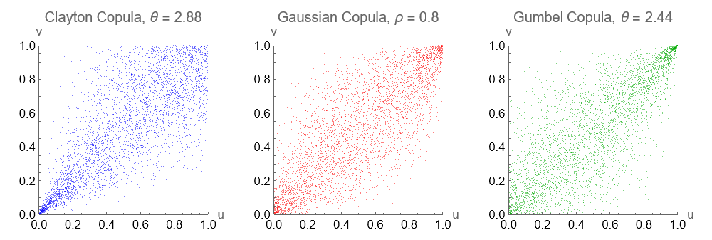
Fig 4.10.1: Scatterplots of pseudo-observations from the Clayton copula ( $\theta=2.88$ ), Gaussian copula ( $\rho=0.8$ ), and Gumbel copula ( $\theta=2.44$ ).

In Figure 4.10.1 we plot three such scatterplots generated by the Mathematica code given in Example A.0.9 in the Appendix. These illustrate how different copulas, even with the same margins and similar Kendall’s $\tau$ , can encode very different dependence structures, particularly in the tails (Joe, 1997; Nelsen, 1999).

7.6 Inference for Copula Models

Suppose that $(X_1,Y_1),\dots,(X_n,Y_n)$ is a random sample from a distribution with continuous marginals $F_X,F_Y$ and copula $C_\theta$ indexed by a parameter $\theta$ . The likelihood for $(X,Y)$ decomposes into marginal and copula parts, paralleling the decomposition of models into components that underlies the likelihood principle in Chapter 6 of Casella & Berger (2002), see, for example, Joe (1997).

Because the copula is invariant under strictly increasing transformations of the margins, it is natural to base inference about $\theta$ on the ranks (or, equivalently, on empirical versions of $U_i=F_X(X_i)$ and $V_i=F_Y(Y_i)$ ). Let $R_i$ and $S_i$ be the ranks of $X_i$ and $Y_i$ among $X_1,\dots,X_n$ and $Y_1,\dots,Y_n$ , respectively. The empirical copula is defined on $[0,1]^2$ by $C_n(u,v) =\frac{1}{n} \sum_{i=1}^n \mathbf{1}\Bigl(\frac{R_i}{n+1}\le u,\frac{S_i}{n+1}\le v\Bigr).$

This is a rank-based estimator of $C$ ; under mild conditions, $C_n(u,v)\to C(u,v)$ for each fixed $(u,v)$ (Genest & Favre, 2007). The use of ranks parallels the rank-based procedures for nonparametric inference introduced in Chapter 8 of Casella & Berger (2002).

Although full maximum likelihood estimation is certainly possible, it could be numerically unstable. Several other rank-based estimation strategies are used in practice:

Method of moments via Kendall’s tau or Spearman’s rho. If $\tau=\tau(\theta)$ (or $\rho_S=\rho_S(\theta)$ ) is known in closed form, one can estimate $\theta$ by solving $\tau(\hat\theta)=\hat\tau$ (or $\rho_S(\hat\theta)=\hat\rho_S$ ), where $\hat\tau$ or $\hat\rho_S$ is computed from the sample ranks (Section 7.2 of Casella & Berger (2002)), cf. (Genest & Favre, 2007).
Maximum pseudolikelihood. If the copula has density $c_\theta(u,v)$ , one may maximize $\ell(\theta) =\sum_{i=1}^n \log c_\theta\Bigl(\frac{R_i}{n+1},\frac{S_i}{n+1}\Bigr)$ with respect to $\theta$ . Under suitable conditions, the maximizer $\hat\theta$ is consistent and asymptotically normal, and its large-sample behavior can be analyzed using the methods of Chapter 10 of Casella & Berger (2002), cf. (Joe, 1997).
Two-step methods. One may first estimate marginal parameters by univariate methods (Chapter 7 of Casella & Berger (2002)) and then estimate $\theta$ by maximizing a “copula likelihood” built from the transformed data, but this approach is sensitive to misspecification of the margins (Joe, 1997).

Rank-based methods have the advantage of depending only on the copula and remaining valid under arbitrary strictly increasing marginal transformations, in line with the invariance considerations emphasized in Chapter 6 of Casella & Berger (2002), cf. (Genest & Favre, 2007).

Example 7.6.1 (Estimating a Clayton copula parameter). Suppose $(X_i,Y_i)$ , $i=1,\dots,n$ , is a sample from a model with continuous marginals and Clayton copula $C_\theta(u,v) =\bigl(u^{-\theta}+v^{-\theta}-1\bigr)^{-1/\theta},\qquad \theta>0.$

For this family, Kendall’s tau is a simple function of $\theta$ : $\tau(\theta)=\frac{\theta}{\theta+2}.$ Let $\hat\tau$ be the sample Kendall’s tau computed from the ranks of the data. A method-of-moments estimator of $\theta$ is obtained by solving $\tau(\hat\theta)=\hat\tau$ , which gives $\hat\theta=\frac{2\hat\tau}{1-\hat\tau}.$

This estimator depends only on the copula (through the ranks) and not on the specific marginal distributions, in contrast with likelihood-based estimators that require a full specification of the marginals (Chapter 7 of Casella & Berger (2002)).

Exercises for Section 4.10

4.66

(Copulas and monotone transformations.) Let $(X,Y)$ be continuous with copula $C$ , and let $Z=g(X)$ , $T=h(Y)$ with $g,h$ strictly increasing.

(a): Using the change-of-variables ideas from Section 2.1, express the cdf of $(Z,T)$ in terms of $F_{X,Y}$ .
(b): Show that $(Z,T)$ has the same copula $C$ .
(c): Let $(X,Y)$ be the bivariate normal pair of Example 4.5.3 of Casella & Berger (2002) with correlation $\rho$ . Take $g(x)=e^x$ and $h(y)=e^{3y}$ . Simulate a moderate sample from this model (see Section 5.5 of Casella & Berger (2002)) and compare the scatter plots of $(X,Y)$ and $(Z,T)$ . Explain why the copula, and thus Kendall’s tau, is the same in both cases.

4.67

(PQD and covariance sign.) Suppose $(X,Y)$ is continuous and positively quadrant dependent: $P(X\le x,Y\le y)\ge P(X\le x)P(Y\le y)\quad\text{for all }x,y.$

(a): Express this condition in terms of the copula $C$ .
(b): Show that if $X$ and $Y$ have finite second moments, then $\mathsf{Cov}(X,Y)\ge 0$ (hint: proceed as in the proof of Theorem 2.2.6 of Casella & Berger (2002), but use the PQD condition).
(c): Consider the model of Example 4.5.2 of Casella & Berger (2002), where $X$ and $Y$ are independent exponentials with parameter $\lambda$ (hence $\mathsf{Cov}(X,Y)=0$ ). Modify this model by introducing a Clayton copula with parameter $\theta>0$ while keeping the same exponential marginals. Argue that the resulting pair is PQD, and discuss how the covariance changes.

4.68

(Gaussian copula and tail independence.) Let $(Z_1,Z_2)$ be bivariate normal with correlation $\rho$ (Section 3.3 of Casella & Berger (2002)), and define $U=\Phi(Z_1)$ , $V=\Phi(Z_2)$ .

(a): Argue that the copula of $(U,V)$ is the Gaussian copula $C_\rho$ .
(b): Using the tail dependence formulas in Section 4.10.4, show heuristically that for $|\rho|<1$ , $\lambda_L=\lambda_U=0$ .
(c): Explain in words why this means that even strongly correlated Gaussian models may understate the probability of joint extreme events.

Exercises for Section 7.6

7.67

(Kendall’s $\tau$ and Archimedean copulas.) An Archimedean copula has the form $C(u,v)=\varphi^{-1}(\varphi(u)+\varphi(v)),$ where $\varphi$ is a convex, decreasing generator.

(a): For the Clayton copula with parameter $\theta>0$ , verify that the generator is $\varphi(t)=t^{-\theta}-1$ .
(b): Using the following formula for Kendall’s $\tau$ in terms of the generator $\tau = 1 + 4 \int_0^1 \frac{\varphi(t)}{\varphi'(t)}\,dt,$ derive $\tau(\theta)$ and base an estimator for $\theta$ on it.

7.68

(A complete copula analysis of rainfall and runoff) The following display contains $n=30$ invented paired observations of rainfall $X$ , measured in millimetres, and same-day runoff volume $Y$ , measured in $10^3\,\mathrm{m}^3$ , from substantial rainfall events in a small catchment. For the purposes of this exercise, regard the pairs as an i.i.d. sample from a continuous bivariate distribution. There are no ties.

Invented rainfall–runoff data for Exercise 7.68.

$i$	$x_i$	$y_i$	$i$	$x_i$	$y_i$	$i$	$x_i$	$y_i$
1	34.7	64.1	11	114.2	105.0	21	35.6	58.1
2	26.8	19.1	12	15.5	17.5	22	50.8	20.3
3	42.1	71.1	13	14.5	21.5	23	97.4	87.7
4	12.9	27.3	14	33.3	42.0	24	57.2	117.8
5	20.1	24.8	15	21.1	13.1	25	34.0	17.2
6	73.5	88.3	16	38.1	45.6	26	16.9	33.9
7	111.9	119.3	17	20.3	41.3	27	13.1	11.5
8	15.7	26.9	18	19.1	22.8	28	27.6	17.4
9	14.0	10.6	19	45.6	39.2	29	40.3	110.0
10	37.9	58.3	20	23.8	22.9	30	33.6	42.5

(a): Draw a scatterplot of $(X_i,Y_i)$ . Describe the marginal distributions and the apparent association. Explain why fitting a bivariate normal distribution on the original measurement scale may be questionable.
(b): Compute Pearson’s sample correlation $r$ , Kendall’s sample tau $\widehat\tau$ , and Spearman’s sample rho $\widehat\rho_S$ . Explain why $\widehat\tau$ and $\widehat\rho_S$ are particularly natural summaries in a copula analysis.
(c): Let $R_i$ and $S_i$ denote the ranks of $X_i$ and $Y_i$ , respectively. Construct the pseudo-observations $U_i=\frac{R_i}{n+1},\qquad V_i=\frac{S_i}{n+1},\qquad i=1,\ldots,n.$ Plot the points $(U_i,V_i)$ in the unit square. Explain why this plot, and hence the empirical copula, is unchanged if $X$ and $Y$ are replaced by $\log X$ and $\log Y$ , respectively.
(d): Define the empirical copula by $C_n(u,v)=\frac{1}{n}\sum_{i=1}^n \mathbf{1}\{U_i\leq u,\,V_i\leq v\},\qquad 0\leq u,v\leq1.$ Compute $C_n(0.5,0.5)$ , $C_n(0.8,0.8)$ , and $C_n(0.9,0.9)$ . Compare these values with those of the independence copula $\Pi(u,v)=uv$ .
(e): Fit a Gaussian copula and a Gumbel copula by inversion of Kendall’s tau. Use $\tau_{\mathrm{Gauss}}(\rho)=\frac{2}{\pi}\arcsin(\rho), \qquad -1<\rho<1,$ and $\tau_{\mathrm{Gumbel}}(\theta)=1-\frac{1}{\theta}, \qquad \theta\geq1.$ Obtain the estimates $\widehat\rho_{\tau}$ and $\widehat\theta_{\tau}$ .
(f): Estimate the same two copulas by maximum pseudolikelihood. For a copula density $c_\eta$ , maximize $\ell_n(\eta)=\sum_{i=1}^n \log c_\eta\!\left(\frac{R_i}{n+1},\frac{S_i}{n+1}\right).$ For the Gaussian copula, you may use $c_\rho(u,v)=\frac{\phi_2\!\left(\Phi^{-1}(u),\Phi^{-1}(v);\rho\right)} {\phi\!\left(\Phi^{-1}(u)\right)\phi\!\left(\Phi^{-1}(v)\right)},$ where $\phi$ is the standard normal density and $\phi_2(\,\cdot\,,\,\cdot\,;\rho)$ is the bivariate standard normal density with correlation $\rho$ . For the Gumbel copula $C_\theta(u,v)=\exp\!\left\{-\left[(-\log u)^\theta+(-\log v)^\theta\right]^{1/\theta}\right\}, \qquad \theta\geq1,$ you may evaluate the mixed derivative $c_\theta(u,v)=\partial^2C_\theta(u,v)/ \partial u\,\partial v$ numerically, or use software that implements this density like Mathematica. Report the maximum-pseudolikelihood estimates $\widehat\rho_{\mathrm{MPL}}$ and $\widehat\theta_{\mathrm{MPL}}$ , and compare them with the estimates from part (e).
(g): State the lower- and upper-tail dependence coefficients for each fitted copula. In particular, show that the Gaussian copula has $\lambda_L=\lambda_U=0$ whenever $|\rho|<1$ , whereas the Gumbel copula has $\lambda_L=0,\qquad \lambda_U=2-2^{1/\theta}.$ Explain why copulas with similar fitted values of Kendall’s tau can nevertheless make substantially different assertions about simultaneous extreme rainfall and runoff events.
(h): Using the pseudo-observation plot together with the maximized pseudo-log-likelihoods and the tail-dependence coefficients obtained above, discuss which model is more appropriate for describing the data. Distinguish carefully between overall positive association and upper-tail dependence.
(i): Let $q_X(0.90)$ and $q_Y(0.90)$ be the empirical $0.90$ quantiles of rainfall and runoff. For each fitted copula, estimate $\Pr\{X>q_X(0.90),\,Y>q_Y(0.90)\} =1-0.90-0.90+C(0.90,0.90).$ Compare the resulting estimates with the independence benchmark $0.10^2=0.01$ . Give a practical interpretation in terms of the occurrence of a high-rainfall event together with high runoff.

Acknowledgement

The author thanks Perplexity AI for assistance with English-language editing and with the preparation and refinement of selected Mathematica code snippets. This assistance was limited to matters of presentation, wording, and coding style. Responsibility for the scientific content, mathematical correctness, numerical calculations, and final form of the manuscript rests entirely with the author.

Appendix

Example A.0.9 (Copula Scatterplots) The following Mathematica code generates scatterplots of pseudo-observations from three copula models with comparable overall dependence: a Clayton copula with parameter $\theta=2.88$ , a Gaussian copula with correlation $\rho=0.8$ , and a Gumbel copula with parameter $\theta=2.44$ .

(* ============================================== *)
(* Copula scatterplots: Clayton, Gaussian, Gumbel *)
(* ============================================== *)

SeedRandom[12345];
n = 5000;

(* ---------------------------------------------- *)
(* 1. Clayton copula, parameter theta = 2.88      *)
(* ---------------------------------------------- *)

thetaClayton = 2.88;

(* Correct Clayton sampler using conditional distribution *)
claytonSample[n_, theta_] := Module[{u, w, v},
  u = RandomReal[{0, 1}, n];
  w = RandomReal[{0, 1}, n];
  v = ((w^(1/(1 + theta)) * u)^(-theta) + 1 - u^(-theta))^(-1/theta);
  Transpose[{u, v}]
];

claytonData = claytonSample[n, thetaClayton];

(* ---------------------------------------------- *)
(* 2. Gaussian copula, parameter rho = 0.8        *)
(* ---------------------------------------------- *)

rho = 0.8;
sigma = {{1, rho}, {rho, 1}};

gaussianSample[n_, sigma_] := Module[{z},
  z = RandomVariate[MultinormalDistribution[{0, 0}, sigma], n];
  CDF[NormalDistribution[0, 1], #] & /@ z
];

gaussianData = gaussianSample[n, sigma];

(* ---------------------------------------------- *)
(* 3. Gumbel copula, parameter theta = 2.44       *)
(* ---------------------------------------------- *)

thetaGumbel = 2.44;

(* Positive alpha-stable sampler, alpha = 1/theta *)
positiveStableSample[alpha_] := Module[{V, E},
  V = RandomReal[{0, Pi}, 1][[1]];
  E = RandomVariate[ExponentialDistribution[1]];
  (Sin[alpha V]/(Sin[V])^(1/alpha)) *
   (Sin[(1 - alpha) V]/E)^((1 - alpha)/alpha)
];

(* Marshall-Olkin sampler for Gumbel copula *)
gumbelSample[n_, theta_] := Module[{alpha, s, e1, e2, u, v},
  alpha = 1/theta;
  Table[
    s = positiveStableSample[alpha];
    e1 = RandomVariate[ExponentialDistribution[1]];
    e2 = RandomVariate[ExponentialDistribution[1]];
    u = Exp[-(e1/s)^alpha];
    v = Exp[-(e2/s)^alpha];
    {u, v},
    {n}
  ]
];

gumbelData = gumbelSample[n, thetaGumbel];

(* ---------------------------------------------- *)
(* 4. Scatterplots                                *)
(* ---------------------------------------------- *)

plotStyle[color_] := Directive[color, PointSize[0.0025], Opacity[0.5]];

claytonPlot = ListPlot[
  claytonData,
  PlotRange -> {{0, 1}, {0, 1}},
  AspectRatio -> 1,
  PlotStyle -> plotStyle[Blue],
  AxesLabel -> {"u", "v"},
  PlotLabel -> "Clayton Copula, \[Theta] = 2.88",
  ImageSize -> 350
];

gaussianPlot = ListPlot[
  gaussianData,
  PlotRange -> {{0, 1}, {0, 1}},
  AspectRatio -> 1,
  PlotStyle -> plotStyle[Red],
  AxesLabel -> {"u", "v"},
  PlotLabel -> "Gaussian Copula, \[Rho] = 0.8",
  ImageSize -> 350
];

gumbelPlot = ListPlot[
  gumbelData,
  PlotRange -> {{0, 1}, {0, 1}},
  AspectRatio -> 1,
  PlotStyle -> plotStyle[Darker[Green]],
  AxesLabel -> {"u", "v"},
  PlotLabel -> "Gumbel Copula, \[Theta] = 2.44",
  ImageSize -> 350
];

GraphicsRow[{claytonPlot, gaussianPlot, gumbelPlot}, Spacings -> 20]

Solutions

Solution to 4.66.

Let $(X,Y)$ be a continuous bivariate random vector with joint cdf $F_{X,Y}$ and copula $C$ , and let $g,h:\mathbb{R}\to\mathbb{R}$ be strictly increasing functions. Define $Z = g(X),\qquad T = h(Y).$

(a) Cdf of $(Z,T)$ in terms of $F_{X,Y}$ .

For any $z,t\in\mathbb{R}$ , $\begin{aligned} F_{Z,T}(z,t) &= \mathbb{P}(Z \le z,\; T \le t) \\ &= \mathbb{P}\bigl(g(X) \le z,\; h(Y) \le t\bigr). \end{aligned}$ Since $g$ and $h$ are strictly increasing, the inequalities $g(X)\le z$ and $h(Y)\le t$ are equivalent to $X \le g^{-1}(z),\qquad Y \le h^{-1}(t),$ where $g^{-1}$ and $h^{-1}$ denote the (strictly increasing) inverses of $g$ and $h$ . Hence $F_{Z,T}(z,t) = \mathbb{P}\bigl(X \le g^{-1}(z),\; Y \le h^{-1}(t)\bigr) = F_{X,Y}\bigl(g^{-1}(z),\,h^{-1}(t)\bigr).$

(b) Copula of $(Z,T)$ .

Let $F_X$ and $F_Y$ be the marginal cdfs of $X$ and $Y$ , and let $F_Z$ and $F_T$ be the marginal cdfs of $Z$ and $T$ . From part (a), $\begin{aligned} F_Z(z) &= \mathbb{P}(Z \le z) = \mathbb{P}\bigl(g(X) \le z\bigr) = \mathbb{P}\bigl(X \le g^{-1}(z)\bigr) = F_X\bigl(g^{-1}(z)\bigr), \\ F_T(t) &= \mathbb{P}(T \le t) = \mathbb{P}\bigl(h(Y) \le t\bigr) = \mathbb{P}\bigl(Y \le h^{-1}(t)\bigr) = F_Y\bigl(h^{-1}(t)\bigr). \end{aligned}$

Let $u,v\in(0,1)$ and define $z = F_Z^{-1}(u),\qquad t = F_T^{-1}(v).$ Using $F_Z(z)=F_X(g^{-1}(z))$ and the strict monotonicity of $g$ , $F_X\bigl(g^{-1}(z)\bigr) = u \quad\Longrightarrow\quad g^{-1}(z) = F_X^{-1}(u),$ so that $z = g\bigl(F_X^{-1}(u)\bigr).$ Similarly, $t = h\bigl(F_Y^{-1}(v)\bigr).$

The copula $C_{Z,T}$ of $(Z,T)$ is defined by $C_{Z,T}(u,v) = F_{Z,T}\bigl(F_Z^{-1}(u),\,F_T^{-1}(v)\bigr).$ Using part (a) and the relations above, $\begin{aligned} C_{Z,T}(u,v) &= F_{Z,T}(z,t) \\ &= F_{X,Y}\bigl(g^{-1}(z),\,h^{-1}(t)\bigr) \\ &= F_{X,Y}\bigl(F_X^{-1}(u),\,F_Y^{-1}(v)\bigr). \end{aligned}$ By definition of the copula $C$ of $(X,Y)$ , $C(u,v) = F_{X,Y}\bigl(F_X^{-1}(u),\,F_Y^{-1}(v)\bigr),$ hence $C_{Z,T}(u,v) = C(u,v),\qquad (u,v)\in[0,1]^2.$ Therefore $(Z,T)$ has the same copula $C$ as $(X,Y)$ .

(c) Bivariate normal example and invariance of the copula.

Let $(X,Y)$ be bivariate normal with correlation $\rho$ , as in Example 4.5.3 of Casella & Berger (2002), and define $Z = g(X) = e^{X},\qquad T = h(Y) = e^{3Y}.$ To simulate a sample of size $n$ from this model, one can:

Generate $n$ i.i.d. observations $(X_i,Y_i)$ from the bivariate normal distribution with correlation $\rho$ .
For each $i$ , set $Z_i = e^{X_i},\qquad T_i = e^{3Y_i}.$

The scatter plot of $(Z_i,T_i)$ is obtained from that of $(X_i,Y_i)$ by applying strictly increasing transformations in each coordinate. These change the marginal distributions (normal to lognormal and scaled lognormal) and the scale of the axes, but they preserve the ordering of the points in each coordinate and hence the dependence structure encoded by the copula.

Part (b) shows rigorously that strictly increasing transformations in each margin leave the copula unchanged. Kendall’s tau is a measure of concordance that depends only on the copula (it is invariant under strictly increasing transformations of each coordinate). Therefore $(X,Y)$ and $(Z,T)$ have the same copula and the same value of Kendall’s tau; empirically, the estimated tau from the two scatter plots will (up to sampling error) be equal.

Solution to 4.67.

Assume $(X,Y)$ is continuous with joint cdf $F_{X,Y}$ , marginals $F_X,F_Y$ , and copula $C$ .

(a) PQD in terms of the copula.

Positive quadrant dependence (PQD) means $P(X\le x,Y\le y)\;\ge\;P(X\le x)\,P(Y\le y)\quad\text{for all }x,y\in\mathbb{R}.$ In terms of the cdfs this is $F_{X,Y}(x,y)\;\ge\;F_X(x)\,F_Y(y)\quad\forall x,y.$ By Sklar’s theorem, $F_{X,Y}(x,y)=C\bigl(F_X(x),F_Y(y)\bigr).$ Let $u=F_X(x)$ and $v=F_Y(y)$ ; then $u,v\in[0,1]$ and the PQD condition becomes $C(u,v)\;\ge\;uv\quad\text{for all }(u,v)\in[0,1]^2.$ Thus $(X,Y)$ is PQD if and only if its copula $C$ satisfies $C(u,v)\ge uv$ on $[0,1]^2$ .

(b) PQD implies nonnegative covariance.

Assume $X$ and $Y$ have finite second moments. We show $\mathsf{Cov}(X,Y)\ge0$ . Recall that for square–integrable $(X,Y)$ one can write $\mathsf{Cov}(X,Y) = \mathbb{E}(XY)-\mathbb{E}X\,\mathbb{E}Y = \iint_{\mathbb{R}^2} \bigl\{P(X>x,Y>y)-P(X>x)\,P(Y>y)\bigr\}\,dx\,dy,$ which is obtained by expanding $XY$ into indicator integrals and interchanging expectation and integration (as in the proof of Theorem 2.2.6).

Note that $P(X>x,Y>y) = 1-F_X(x)-F_Y(y)+F_{X,Y}(x,y),$ and $P(X>x)\,P(Y>y) = (1-F_X(x))(1-F_Y(y)) = 1-F_X(x)-F_Y(y)+F_X(x)F_Y(y).$ Hence $P(X>x,Y>y)-P(X>x)\,P(Y>y) = F_{X,Y}(x,y)-F_X(x)F_Y(y).$ Therefore $\mathsf{Cov}(X,Y) = \iint_{\mathbb{R}^2} \bigl(F_{X,Y}(x,y)-F_X(x)F_Y(y)\bigr)\,dx\,dy.$

If $(X,Y)$ is PQD, then $F_{X,Y}(x,y)\ge F_X(x)F_Y(y)$ for all $x,y$ , so the integrand is everywhere nonnegative. The integral of a nonnegative function is nonnegative, hence $\mathsf{Cov}(X,Y)\;\ge\;0.$

(c) Clayton copula with exponential marginals.

In Example 4.5.2, $X$ and $Y$ are independent exponentials with parameter $\lambda$ : $F_X(x)=F_Y(x)=1-e^{-\lambda x},\qquad x\ge0,$ and $F_{X,Y}(x,y)=F_X(x)F_Y(y) \quad\Rightarrow\quad \mathsf{Cov}(X,Y)=0.$

Now keep these marginals but introduce dependence via a Clayton copula with parameter $\theta>0$ : $C_\theta(u,v) = \left(u^{-\theta}+v^{-\theta}-1\right)^{-1/\theta}, \qquad u,v\in(0,1],\;\theta>0.$ The joint cdf of the new pair $(X_\theta,Y_\theta)$ is $F_{X_\theta,Y_\theta}(x,y) = C_\theta\bigl(F_X(x),F_Y(y)\bigr),\qquad x,y\ge0.$

PQD: For Clayton copulas with $\theta>0$ one has $C_\theta(u,v)\;\ge\;uv,\qquad (u,v)\in[0,1]^2.$ Thus the copula $C_\theta$ lies above the independence copula $uv$ , so by part (a) the resulting pair $(X_\theta,Y_\theta)$ is positively quadrant dependent.

Covariance: By part (b), PQD and finite second moments imply $\mathsf{Cov}(X_\theta,Y_\theta)\;\ge\;0.$ When $\theta = 0$ (interpreted as a limit), the copula reduces to the product copula $uv$ , i.e. independence, so $\operatorname{Cov}(X_0,Y_0)=0.$ For $\theta>0$ , the resulting pair is positively quadrant dependent and hence has nonnegative covariance. Increasing $\theta$ corresponds to stronger positive dependence within the Clayton family. Thus introducing a Clayton copula with parameter $\theta>0$ , while keeping the exponential marginals, turns the originally independent pair into a positively quadrant dependent pair with nonnegative covariance.

Solution to 4.68.

Let $(Z_1,Z_2)$ be bivariate normal with correlation $\rho$ , and let $U=\Phi(Z_1),\qquad V=\Phi(Z_2),$ where $\Phi$ is the standard normal cdf.

(a) Copula of $(U,V)$ .

By construction, $U = F_{Z_1}(Z_1),\qquad V = F_{Z_2}(Z_2),$ where $F_{Z_i}=\Phi$ are the marginal cdfs of $Z_i$ . Thus $U$ and $V$ are standard uniform random variables (probability integral transform). Their joint cdf is $\begin{aligned} P(U\le u, V\le v) &= P\bigl(\Phi(Z_1)\le u,\ \Phi(Z_2)\le v\bigr) \\ &= P\bigl(Z_1\le \Phi^{-1}(u),\ Z_2\le \Phi^{-1}(v)\bigr) \\ &= F_{(Z_1,Z_2)}\bigl(\Phi^{-1}(u),\Phi^{-1}(v)\bigr), \end{aligned}$ where $F_{(Z_1,Z_2)}$ is the bivariate normal cdf with correlation $\rho$ . By definition, the copula $C_\rho$ associated with this bivariate normal distribution is $C_\rho(u,v) := F_{(Z_1,Z_2)}\bigl(\Phi^{-1}(u),\Phi^{-1}(v)\bigr).$ Comparing the two displays, we see that $(U,V)$ has copula $C_\rho$ (the Gaussian copula with parameter $\rho$ ).

(b) Tail dependence for $|\rho|<1$ .

Recall the upper and lower tail dependence coefficients for a copula $C$ : $\lambda_U = \lim_{u\uparrow 1} \frac{1 - 2u + C(u,u)}{1-u}, \qquad \lambda_L = \lim_{u\downarrow 0} \frac{C(u,u)}{u}.$

For the Gaussian copula $C_\rho$ , we have $C_\rho(u,u) = P(U\le u, V\le u) = P\bigl(Z_1\le z,\ Z_2\le z\bigr), \quad\text{where }z=\Phi^{-1}(u).$ Equivalently, $P(Z_1>z, Z_2>z) = 1 + C_\rho(u,u) - 2u.$

Upper tail. Write $P(U>u, V>u) = P(Z_1>z, Z_2>z), \quad u\to 1,\;z\to\infty.$ For a bivariate normal with $|\rho|<1$ , it is known (and can be derived via asymptotic analysis of the joint normal tail) that $P(Z_1>z, Z_2>z) \sim k(\rho)\,\frac{1}{z}\exp\!\left(-\frac{z^2}{1+\rho}\right), \qquad z\to\infty,$ for some positive constant $k(\rho)$ depending on $\rho$ . On the other hand, $P(Z_1>z) = 1-u \sim \frac{1}{z}\exp\!\left(-\frac{z^2}{2}\right), \qquad z\to\infty.$ Therefore $\frac{P(Z_1>z, Z_2>z)}{P(Z_1>z)} \sim k(\rho)\exp\!\left(-z^2\left[\frac{1}{1+\rho} - \frac{1}{2}\right]\right).$ If $|\rho|<1$ , then $\frac{1}{1+\rho} > \frac{1}{2}$ , so the exponent is negative and the ratio decays to $0$ as $z\to\infty$ . Translating back to the copula formulation, this means $\lambda_U = \lim_{u\uparrow 1} P(U>u\mid V>u) = 0,\qquad |\rho|<1.$

Lower tail. By symmetry of the bivariate normal about $(0,0)$ , $(Z_1,Z_2)$ and $(-Z_1,-Z_2)$ have the same joint distribution (with the same correlation $\rho$ ). Thus lower–tail events $(Z_1\le -z, Z_2\le -z)$ correspond to upper–tail events for $(-Z_1,-Z_2)$ ; the same asymptotic analysis applies and yields $\lambda_L = 0,\qquad |\rho|<1.$

Heuristically, for any fixed $\rho$ strictly less than $1$ in magnitude, the joint tail of the bivariate normal decays faster than the marginal tail, so the conditional probability of a joint extreme given a marginal extreme goes to zero in both tails.

(c) Interpretation for joint extremes.

The fact that $\lambda_L=\lambda_U=0$ for $|\rho|<1$ means that, in a Gaussian copula model, the probability of observing one variable in an extreme tail given that the other is in that tail tends to $0$ as we move further into the tail. In other words, even if the linear correlation $\rho$ is large (say $\rho=0.9$ ), the Gaussian dependence structure does not create asymptotic clustering of extremes: very large values of $X$ and $Y$ do not tend to occur together with positive limiting probability.

In practical terms, this implies that strongly correlated Gaussian models can substantially understate the probability of joint extreme events. They may fit well in the center of the distribution (capturing linear correlation), but they impose tail independence: extreme events in one margin are, asymptotically, almost never accompanied by simultaneous extremes in the other margin. For applications where joint tail behavior is critical (e.g. financial or environmental risk), the Gaussian copula may therefore give overly optimistic (too small) estimates of joint extreme risks.

Solution to 7.67

An Archimedean copula has the form $C(u,v) = \varphi^{-1}\bigl(\varphi(u)+\varphi(v)\bigr),$ where $\varphi$ is a convex, decreasing generator.

(a): Clayton generator.; The (bivariate) Clayton copula with parameter $\theta>0$ is $C_\theta(u,v) = \left(u^{-\theta}+v^{-\theta}-1\right)^{-1/\theta}, \qquad u,v\in(0,1].$; We claim that this can be written in Archimedean form with generator $\varphi(t) = t^{-\theta} - 1,\qquad t\in(0,1].$; First compute its inverse: $s = \varphi(t) = t^{-\theta} - 1 \quad\Longrightarrow\quad t^{-\theta} = s+1 \quad\Longrightarrow\quad t = (1+s)^{-1/\theta}.$ Hence $\varphi^{-1}(s) = (1+s)^{-1/\theta},\qquad s\ge0.$; Now form the Archimedean copula associated with this generator: $C(u,v) = \varphi^{-1}\bigl(\varphi(u)+\varphi(v)\bigr) = \Bigl( 1 + (u^{-\theta}-1) + (v^{-\theta}-1) \Bigr)^{-1/\theta} = \bigl(u^{-\theta} + v^{-\theta} - 1\bigr)^{-1/\theta}.$; This is exactly the (alternative) Archimedean representation of the Clayton copula, so $\varphi(t)=t^{-\theta}-1$ is indeed a valid generator for the Clayton family.
(b): Kendall’s $\tau$ and an estimator for $\theta$ .; For an Archimedean copula with generator $\varphi$ , Kendall’s $\tau$ is given by $\tau = 1 + 4\int_0^1 \frac{\varphi(t)}{\varphi'(t)}\,dt.$; For $\varphi(t)=t^{-\theta}-1$ we have $\varphi'(t) = -\theta t^{-\theta-1}.$ Therefore $\frac{\varphi(t)}{\varphi'(t)} = \frac{t^{-\theta}-1}{-\theta t^{-\theta-1}} = -\frac{1}{\theta}\,(t - t^{\theta+1}).$; Plugging into the formula for $\tau$ , $\tau(\theta) = 1 + 4\int_0^1 \frac{\varphi(t)}{\varphi'(t)}\,dt = 1 + 4\int_0^1 \left(-\frac{1}{\theta}(t - t^{\theta+1})\right)\!dt = 1 - \frac{4}{\theta}\int_0^1 (t - t^{\theta+1})\,dt.$; Compute the integral: $\int_0^1 t\,dt = \frac{1}{2}, \qquad \int_0^1 t^{\theta+1}\,dt = \frac{1}{\theta+2}.$ Hence $\int_0^1 (t - t^{\theta+1})\,dt = \frac{1}{2} - \frac{1}{\theta+2} = \frac{\theta}{2(\theta+2)}.$; Substitute back: $\tau(\theta) = 1 - \frac{4}{\theta}\cdot\frac{\theta}{2(\theta+2)} = 1 - \frac{2}{\theta+2} = \frac{\theta}{\theta+2}.$; Thus Kendall’s $\tau$ for this Clayton copula (with generator $\varphi(t)=t^{-\theta}-1$ ) is $\boxed{\tau(\theta) = \frac{\theta}{\theta+2}}.$; To base an estimator for $\theta$ on Kendall’s $\tau$ , let $\hat\tau$ denote the sample (empirical) Kendall’s $\tau$ . We invert the above relationship: $\hat\tau = \frac{\theta}{\theta+2} \quad\Longrightarrow\quad \hat\tau(\theta+2) = \theta \quad\Longrightarrow\quad \theta(1 - \hat\tau) = 2\hat\tau \quad\Longrightarrow\quad \boxed{\hat\theta = \frac{2\hat\tau}{1-\hat\tau}}.$; This $\hat\theta$ is the method-of-moments–type estimator of the Clayton parameter based on Kendall’s $\tau$ .

Solution to 7.68

Write $n=30$ . The data are listed in random observation order; that order has no statistical significance. There are no ties. In the copula calculations below, we use the rank pseudo-observations $U_i=\frac{R_i}{n+1}=\frac{R_i}{31},\qquad V_i=\frac{S_i}{n+1}=\frac{S_i}{31},\qquad i=1,\ldots,30.$

(a): The scatterplot shows a clear positive association, but it is far from a deterministic functional relationship. There is substantial variation in runoff at comparable rainfall amounts; for example, the observations with rainfall near $34$ – $40$ mm have runoff values ranging from about $17$ to $110$ in the stated units. This is plausible because runoff also depends on antecedent wetness, rainfall intensity and duration, catchment storage, routing, and measurement variation.; Both variables are positive and right-skewed. Consequently, a bivariate normal model on the original scale is unattractive: normal margins are symmetric and place positive probability on negative rainfall and runoff. Logarithmic transformations may improve marginal plots, but they do not change the copula, because they are strictly increasing on the positive half-line.
(b): The numerical summaries are $r=0.7948,\qquad \widehat\tau=0.5540,\qquad \widehat\rho_S=0.7339.$ Thus the sample displays moderately strong positive association. Pearson’s $r$ measures linear association on the original measurement scales and can change under nonlinear increasing transformations. In contrast, Kendall’s tau and Spearman’s rho depend only on the joint ranks and hence are invariant under strictly increasing transformations of either margin. This makes them especially natural for a copula analysis.
(c): The rank pseudo-observations are obtained from the following ranks: $\begin{array}{c|rrrrrrrrrr} i&1&2&3&4&5&6&7&8&9&10\\ \hline R_i&18&13&23&1&9&27&29&6&3&20\\ S_i&23&7&24&14&12&26&30&13&1&22 \end{array}$ $\begin{array}{c|rrrrrrrrrr} i&11&12&13&14&15&16&17&18&19&20\\ \hline R_i&30&5&4&15&11&21&10&8&24&12\\ S_i&27&6&9&18&3&20&17&10&16&11 \end{array}$ $\begin{array}{c|rrrrrrrrrr} i&21&22&23&24&25&26&27&28&29&30\\ \hline R_i&19&25&28&26&17&7&2&14&22&16\\ S_i&21&8&25&29&4&15&2&5&28&19 \end{array}$ The plot of $(U_i,V_i)$ in the unit square shows positive rank association with appreciable scatter. If rainfall and runoff are replaced by $\log X$ and $\log Y$ , respectively, their ranks do not change because the logarithm is strictly increasing. Therefore neither the pseudo-observations nor the empirical copula changes.
(d): Direct counting yields $C_n(0.5,0.5)=\frac{13}{30}=0.4333, \quad C_n(0.8,0.8)=\frac{23}{30}=0.7667, \quad C_n(0.9,0.9)=\frac{25}{30}=0.8333.$ Under independence, the corresponding values are $\Pi(0.5,0.5)=0.25,\qquad \Pi(0.8,0.8)=0.64,\qquad \Pi(0.9,0.9)=0.81.$ The empirical copula exceeds the independence copula at all three selected points, which is consistent with positive quadrant dependence in the sample. The comparison at $(0.9,0.9)$ must be interpreted cautiously: with only 30 observations, very few data points concern the most extreme part of the unit square.
(e): Inversion of the stated Kendall-tau relationships gives $\widehat\rho_{\tau} =\sin\left(\frac{\pi\widehat\tau}{2}\right) =0.7645,$ and $\widehat\theta_{\tau} =\frac{1}{1-\widehat\tau} =2.2423.$ Thus both copulas are fitted to the same global rank-dependence summary.
(f): Maximizing the rank-based pseudo-log-likelihood gives, numerically, $\widehat{\rho}_{\mathrm{MPL}}=0.7707, \qquad \widehat{\theta}_{\mathrm{MPL}}=2.2446.$ At their respective maxima, the pseudo-log-likelihood values are approximately $\ell_{\mathrm{Gauss}}=11.4359, \qquad \ell_{\mathrm{Gumbel}}=12.1508.$ The two estimation methods give broadly similar dependence levels. For this sample, the fitted Gumbel copula has the larger maximized pseudo-log-likelihood. This comparison is descriptive; with $n=30$ , it should not be interpreted as decisive evidence for an upper-tail-dependent model.
(g): For every Gaussian copula with $|\rho|<1$ , $\lambda_L=\lambda_U=0.$ For a Gumbel copula, $\lambda_L=0, \qquad \lambda_U=2-2^{1/\theta}.$ Using the maximum-pseudolikelihood estimate yields $\widehat{\lambda}_U = 2-2^{1/\widehat{\theta}_{\mathrm{MPL}}} = 2-2^{1/2.2446} \approx0.6382.$ Using the inversion-of-tau estimate instead gives $2-2^{1/2.2423}\approx0.6378.$; Hence the Gaussian and Gumbel copulas can describe broadly comparable ordinary rank association while making different assertions about extreme events. The Gaussian copula is asymptotically tail independent: as the threshold tends to one, joint exceedances become negligible relative to a marginal exceedance. The Gumbel copula retains positive upper-tail dependence.
(h): The pseudo-observations show a broadly increasing cloud rather than a concentration exactly on the diagonal. Both fitted families capture this central positive association reasonably well. The Gumbel copula is substantively attractive when joint high rainfall and high runoff are the principal scientific concern because it permits upper-tail dependence. Moreover, for this sample its maximized pseudo-log-likelihood, $\ell_{\mathrm{Gumbel}}=12.1508,$ is slightly larger than that of the Gaussian copula, $\ell_{\mathrm{Gauss}}=11.4359.$ Thus the Gumbel copula is the preferred model among these two fitted families on this descriptive criterion. Nevertheless, with only $n=30$ observations, the data provide limited information in the extreme upper-right corner of the unit square. The preference for Gumbel should therefore be interpreted cautiously and not as conclusive evidence of asymptotic upper-tail dependence.
(i): For $q=0.90$ , the fitted-copula estimates are $\widehat p_{\mathrm{Gauss}} = 1-2q+C_{\widehat{\rho}_{\mathrm{MPL}}}(q,q) \approx0.0532,$ and $\widehat p_{\mathrm{Gumbel}} = 1-2q+C_{\widehat{\theta}_{\mathrm{MPL}}}(q,q) \approx0.0663.$ Both are substantially greater than the independence benchmark $0.10^2=0.01.$ The Gumbel copula gives the larger estimated probability of coincident high rainfall and high runoff. Its distinction from the Gaussian copula becomes still more consequential when extrapolating to more extreme thresholds, because it has positive upper-tail dependence whereas the Gaussian copula is asymptotically tail independent.

Mathematica code snippets. The code below reproduces the calculations. It is written using elementary built-in functions. Numerical optimization is restricted to the interior of the parameter spaces because the copula densities are singular or problematic at the boundaries.

(* --------------------------------------------------------------- *)
(* 1. Data, scatterplots, ranks, and pseudo-observations           *)
(* --------------------------------------------------------------- *)
data = {
  {34.7, 64.1}, {26.8, 19.1}, {42.1, 71.1}, {12.9, 27.3},
  {20.1, 24.8}, {73.5, 88.3}, {111.9, 119.3}, {15.7, 26.9},
  {14.0, 10.6}, {37.9, 58.3}, {114.2, 105.0}, {15.5, 17.5},
  {14.5, 21.5}, {33.3, 42.0}, {21.1, 13.1}, {38.1, 45.6},
  {20.3, 41.3}, {19.1, 22.8}, {45.6, 39.2}, {23.8, 22.9},
  {35.6, 58.1}, {50.8, 20.3}, {97.4, 87.7}, {57.2, 117.8},
  {34.0, 17.2}, {16.9, 33.9}, {13.1, 11.5}, {27.6, 17.4},
  {40.3, 110.0}, {33.6, 42.5}
  };

{x, y} = Transpose[data];
n = Length[data];

ListPlot[data, Frame -> True, PlotRange -> All,
 FrameLabel -> {"rainfall (mm)", "runoff (10^3 m^3)"},
 PlotStyle -> Directive[Blue, PointSize[0.016]]]

(* Because there are no ties, Ordering[Ordering[...]] gives ranks. *)
rX = Ordering[Ordering[x]];
rY = Ordering[Ordering[y]];
u = N[rX/(n + 1)];
v = N[rY/(n + 1)];
uv = Transpose[{u, v}];

ListPlot[uv, Frame -> True, AspectRatio -> 1,
 FrameLabel -> {"u", "v"}, PlotRange -> {{0, 1}, {0, 1}},
 PlotStyle -> Directive[Red, PointSize[0.016]]]

(* --------------------------------------------------------------- *)
(* 2. Pearson correlation, Spearman rho, and Kendall tau           *)
(* --------------------------------------------------------------- *)
rPearson = Correlation[x, y];

(* Spearman rho, valid because there are no ties. *)
rhoSHat = 1 - 6 Total[(rX - rY)^2]/(n (n^2 - 1));

(* Kendall tau: concordant minus discordant pairs, divided by n choose 2. *)
pairs = Subsets[Range[n], {2}];
tauHat = Total[Sign[(x[[#[[1]]]] - x[[#[[2]]]])*
                     (y[[#[[1]]]] - y[[#[[2]]]])] & /@ pairs]/Binomial[n, 2];

N[{rPearson, tauHat, rhoSHat}]
(* {0.794774, 0.554023, 0.733927} *)

(* --------------------------------------------------------------- *)
(* 3. Empirical copula and inversion of Kendall's tau               *)
(* --------------------------------------------------------------- *)
empCopula[a_?NumericQ, b_?NumericQ] := 
  Total[
    Boole[#1 <= a && #2 <= b] & @@@ Transpose[{u, v}]
  ]/n;

N[empCopula @@@ {{.5, .5}, {.8, .8}, {.9, .9}}]
(* {0.433333, 0.766667, 0.833333} *)

rhoTau = Sin[Pi tauHat/2];
thetaTau = 1/(1 - tauHat);
N[{rhoTau, thetaTau}]
(* {0.764495, 2.24227} *)

(* --------------------------------------------------------------- *)
(* 4. Copula densities and maximum pseudolikelihood                *)
(* --------------------------------------------------------------- *)
gaussianDensity[uu_?NumericQ, vv_?NumericQ, rho_?NumericQ] :=
 Module[{a, b},
  a = InverseCDF[NormalDistribution[], uu];
  b = InverseCDF[NormalDistribution[], vv];
  Exp[(2 rho a b - rho^2 (a^2 + b^2))/(2 (1 - rho^2))]/
   Sqrt[1 - rho^2]
  ];

gumbelDensity[uu_?NumericQ, vv_?NumericQ, theta_?NumericQ] :=
 Module[{a, b, s, t},
  a = -Log[uu];
  b = -Log[vv];
  s = a^theta + b^theta;
  t = s^(1/theta);
  Exp[-t] (a b)^(theta - 1) s^(1/theta - 2) (t + theta - 1)/(uu vv)
  ];

logLikGaussian[rho_?NumericQ] :=
 Total[Log[gaussianDensity[#[[1]], #[[2]], rho]] & /@ uv];

logLikGumbel[theta_?NumericQ] :=
 Total[Log[gumbelDensity[#[[1]], #[[2]], theta]] & /@ uv];

fitGaussian = FindMaximum[
 {logLikGaussian[rho], -.999 < rho < .999}, {rho, rhoTau}];

fitGumbel = FindMaximum[
 {logLikGumbel[theta], 1.000001 < theta < 20}, {theta, thetaTau}];

N[{fitGaussian, fitGumbel}]
(* {{11.4359, {rho -> 0.770723}},
    {12.1508, {theta -> 2.24462}}} *)

(* --------------------------------------------------------------- *)
(* 5. Tail dependence and fitted joint exceedance probability       *)
(* --------------------------------------------------------------- *)
rhoMPL = rho /. Last[fitGaussian];
thetaMPL = theta /. Last[fitGumbel];

lambdaLGaussian = 0;
lambdaUGaussian = 0;
lambdaLGumbel = 0;
lambdaUGumbel = 2 - 2^(1/thetaMPL);
N[lambdaUGumbel]
(* 0.638205 *)

gaussianCopula[q_?NumericQ, rho_?NumericQ] := CDF[
 MultinormalDistribution[{0, 0}, {{1, rho}, {rho, 1}}],
 {InverseCDF[NormalDistribution[], q],
  InverseCDF[NormalDistribution[], q]}];

gumbelCopula[q_?NumericQ, theta_?NumericQ] :=
 Exp[-(2 (-Log[q])^theta)^(1/theta)];

q = .90;
pGauss = 1 - 2 q + gaussianCopula[q, rhoMPL];
pGumbel = 1 - 2 q + gumbelCopula[q, thetaMPL];
N[{pGauss, pGumbel}]
(* {0.053241, 0.0663387} *)

Note that the population data-generating mechanism used to create this teaching sample was a Gumbel copula with $\theta_0=2.5$ , for which $\tau_0=0.60$ and $\lambda_U=2-2^{1/2.5}\approx0.68$ , combined with lognormal margins. The realized sample need not reproduce the generating parameter exactly; in fact, its moderate size is useful for illustrating sampling variation and the limits of tail-dependence inference from a small dataset.

References

Casella, G., & Berger, R. L. (2002). Statistical inference (2nd ed.). Duxbury.
Genest, C., & Favre, A.-C. (2007). Everything You Always Wanted to Know about Copula Modeling but Were Afraid to Ask. Journal of Hydrologic Engineering, 12(4), 347–368. https://doi.org/10.1061/(asce)1084-0699(2007)12:4(347)
Joe, H. (1997). Multivariate Models and Multivariate Dependence Concepts. Chapman and Hall/CRC. https://doi.org/10.1201/9780367803896
Nelsen, R. B. (1999). An Introduction to Copulas. In Lecture Notes in Statistics. Springer New York. https://doi.org/10.1007/978-1-4757-3076-0
Salmon, F. (2009). Recipe for disaster: The formula that killed wall street. Wired, 17(3).
Sklar, A. (1959). Fonctions de répartition à n dimensions et leurs marges. Publications de l’Institut de Statistique de l’Université de Paris, 8, 229–231.

Cite this article

Müller, W. (2026). An Introduction to Copulas: a Complement. Journal of Reproducible Statistics, 1, 2. https://doi.org/10.68365/jrepstat.2026.2

doi: https://doi.org/10.68365/jrepstat.2026.2

Downloads

PDF ePub JATS XML .bib .ris .csl.json Reproducibility package (.zip) 25f12f5804da81dee6200eb645fbe1adc96c3fd4437327df78762e13eae71a9f

Once the Crossref deposit is live, https://doi.org/10.68365/jrepstat.2026.2 will also support content negotiation — these exports are served directly regardless.