Department of Mathematical Sciences1, University of Bath, Bath, BA2 7AY, United Kingdom
Abstract
PCR-based measurement of RNA targets in wastewater epidemiology is subject to substantial variation, resulting in considerable uncertainty in disease prevalence estimates. Often, control RNA targets, which are either naturally present or introduced into wastewater samples, are used to normalize the estimated RNA concentration for the primary target. We consider methods for normalization that do not rely on the availability of disease prevalence from public health sources. We demonstrate why direct normalization is unlikely to be effective and may make variation worse. We propose a Kalman filter method for normalization and find that, given the quality of available controls, it offers only limited benefit. We discuss other methods of reducing variation.
Keywords: Wastewater-based surveillance, Normalization, PCR, Controls, Pepper Mild Mottle Virus, Bovine Coronavirus
Wastewater-based surveillanceNormalizationPCRControlsPepper Mild Mottle VirusBovine CoronavirusIntroduction
In wastewater-based epidemiology (WBE), the concentration of a target substance is measured at a wastewater treatment plant (WWTP) to learn about disease prevalence or lifestyle habits in the population in the catchment area of the WWTP. For example, the concentration of SARS-CoV2 RNA might be used to predict the prevalence of Covid-19 in the catchment area. A systematic review of the large literature on wastewater surveillance using SARS-CoV2 RNA may be found in (Deák, Lupu and Prangate, 2026). RNA targets associated with influenza, norovirus and many other diseases are now measured around the world.
We need a precise estimate of the concentration of the RNA in a sample because this is assumed proportional to the number of infected individuals in a WWTP catchment area. Unfortunately, this estimate is subject to three substantive sources of variation. The first source is human-related – the rate at which RNA is excreted over the course of the infection, movement of people in and out of the catchment area etc. – we do not address this here. The second source concerns what happens to the RNA in the sewer between the human and the influent point at the WWTP where the sample is drawn and transported to the laboratory. The third source of variation concerns the preparation, extraction and the PCR measurement that occurs in the laboratory. The methods we discuss here relate mostly to laboratory variation and partly to the sewer variation.
The exponential amplification through the cycles of a PCR measurement unavoidably leads to substantial variation in the estimated concentration of RNA in a sample. A common method for reducing this variation and other sources of variation in the process involves the measurement of a control target which is subject to similar perturbations during the process. There are two kinds of control. One relates to a substance which we assume is excreted at a constant rate by all individuals in the catchment area. Commonly used examples include pepper mild mottle virus (PMMoV) and CrAssphage. These controls will address variation due to the sewer as well as the laboratory. Another type of control is a known fixed quantity of RNA which is added into the sample after collection. Examples of this include porcine reproductive and respiratory syndrome virus and bovine coronavirus (BCoV). Any observed variation in the measurement of these controls can be attributed to at least some parts of the laboratory measurement process. Since we might reasonably assume that the control is subject to many of the same perturbations that apply to the target and will be correlated, we can attempt to use this information using normalization to reduce variation in the target. This type of adjustment is commonplace in applications beyond WBE but there are considerations particular to this situation. A systematic review of normalization methods used in WBE is found in (Ahmed et al., 2026).
Another type of normalization uses information about the sample, such as the ammonia content of the wastewater, that is not directly related to the PCR measurement. This normalization is aimed more at reducing bias than variation. In contrast, the controls are assumed to be approximately constant so normalization using these is focused on variance reduction. Our focus here is variance reduction using controls.
We start with an examination of the most common way of using the control information to adjust the estimate of the target and explain why this method is unlikely to work in the circumstances that are likely to apply. The fundamental objection is that the measurement of the control, which uses the same technology as the measurement of the target, is too variable.
We present a superior method of making the adjustment using the Kalman filter. The methodology is demonstrated on some WBE data from California. We also simulate data with properties like the observed data but with some changed features. These simulations illustrate different scenarios where this method of adjustment is more or less likely to be effective.
Many researchers have used control adjustment where prevalence information about the disease for the targeted pathogen is available. In these situations, one can propose a model of the general form:
Prevalence = f(target RNA, control RNA, other variables)
There is a wide selection of statistical and machine learning models for estimating the function f() that would take advantage of the additional information supplied by the control and other variables. Most examples of this approach have prevalence of COVID19 as the response where this is measured using public health monitoring independent of WBE. For recent examples, see (Darling et al., 2025; Lamm et al., 2025; Verani et al., 2025). This modelling approach usually indicates some predictive value associated with some control variates. Virtually all published research shows some success in predicting the prevalence using the target RNA. While this is encouraging for the utility of WBE, there are some drawbacks.
Many published articles start with the claim that WBE has advantages over standard public health indicators. These articles then proceed to use prevalence data obtained from public health sources to develop their models. For WBE to be truly useful, it must function without requiring public health data. One might argue that models calibrated using prevalence data can subsequently be used to predict prevalence in new situations. Successful extrapolation to different times, locations and targets is uncertain. Published models are often internally validated on their own data but robust external validation in truly new scenarios is problematic. Another difficulty with many published models is that they have been built retrospectively once all the data has been collected. For WBE to be useful as an early warning system, it needs to work in real time.
For these reasons, we focus our attention on methods to normalize the target RNA measure using a control without any public health data. Our aim is to produce an improved RNA-based indicator of disease using auxiliary information but not using the prevalence.
Data
We demonstrate our methods on data used by (Schenk et al., 2024) and presented in (Boehm et al., 2025) where details of the data collection may be found. We focus on a single site, Sunnyvale, California and only three targets: the primary, SARS-CoV2 RNA and two controls, Pepper Mild Mottle Virus (PMMoV) RNA and Bovine Coronavirus (BCoV). The data was collected daily between 1st January 2022 and 30th June 2024, a period of 911 days. The data is high quality, collected daily (excepting 14 missing days), consists of long time series and is publicly available making it a good representative example of current WBE data. Sunnyvale is an ordinary mid-sized city. In the supplementary materials, we compute statistics on the other 190 sites in the data indicating that Sunnyvale is not exceptional. The laboratory method here used wastewater solids whereas other methods use liquid influent. The effectiveness of normalization depends on the joint distribution of the targets. Our main purpose is not to make any specific claims about this chosen dataset, but to address the general problem.
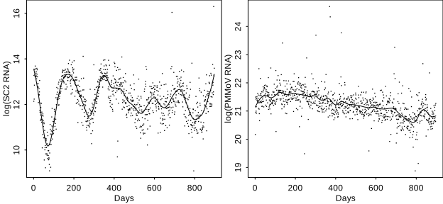
Daily measured SARS-CoV2 and PMMoV RNA in gene copies per gram dry weight on a log scale for 897 days in Sunnyvale, California. Solid line indicates a spline smoothed fit.
Two of the targets are shown in Figure 1. Details of the construction of these plots and subsequent analysis are provided in the supplementary material. We see a clear signal in the SARS-CoV2 although the daily measurement varies considerably around this trend. The RNA counts for PMMoV are about 7,000 times higher than SARS-CoV2. In contrast, the standard deviation of the residuals around the trend for PMMoV is 27% smaller than that seen in SARS-CoV2. PMMoV has a much stronger concentration but can be measured with only modestly greater relative precision. We also see a downward trend in the PMMoV concentration. The trend may be due to external causes such as lower pepper consumption or temporal changes in the sewerage or the measurement process. This has consequences for the normalization but identifying the cause is difficult. This is explored in (Rosengart et al., 2025). However, this problem is not the focus of this article.
Direct Normalization
Suppose we measure a target and a control variable where t is the time index. We assume that the expected value of the control, is constant in and that there are common factors which cause and to positively covary. The mechanisms for this vary according to the type of control variate.
Direct normalization computes:
where could be set to maintain the mean level of by using or similar. This method is widely used in the WBE and other applications. Recent examples include (Sweetapple et al., 2023; Pellett et al., 2024; Schenk et al., 2024). Sometimes more than one control variate is considered.
If and are normally distributed, will have a normal ratio distribution. In the worst case, when and are mean centered, would have a Cauchy distribution. This distribution has notoriously heavy tails and not even its expectation is defined. This would be a terrible choice for an indicator monitoring the prevalence of a disease. One can avoid this pitfall by not mean centering and ensuring that is bounded well away from zero i.e. in practice we must have a strong control that is persistently present at high concentrations. This is true for our Sunnyvale example where no such problems arise. The normal ratio distribution is known for having long tails so outliers may be generated and care must be taken. The properties of this distribution are discussed in (Marsaglia, 2006) who provides formulae to compute the variance of the ratio under different scenarios.
It is more convenient to consider the measurements on a log scale. Furthermore, since the errors are multiplicative, given the nature of PCR, a log scale is even preferable. One can compare unadjusted variance on a log scale, with the comparable adjusted variance using the standard formula for the difference of two random variables:
The correlation between and is given by The c is a constant so does not affect the variance. We see that for variation in the normalized target to be smaller than that in the variation in unnormalized target, the control variation needs to be small and the correlation needs to be large. The problem is that, in WBE applications, T and C are both measured using PCR so the variation in measurement will tend to be similar while the correlation tends to be moderate at best. The adjustment can easily make the variance higher. Some evidence of this is reported in (Darling et al., 2025).
Let’s consider the Sunnyvale data. To estimate and , we need to make some assumptions. In Figure 1, we don’t expect the true value of the SARS-CoV2 measure to vary substantially from one day to the next because
SARS-CoV2 in the wastewater derives from individuals whose COVID infection lasts several days. These individuals contribute a rising then falling amount of SARS-CoV2 RNA over these days.
The number of people infected with COVID will not change extremely rapidly from one day to the next (either up or down)
We are observing a convolution of multiple SARS-CoV2 sources in the wastewater
The reasons that the RNA measures vary so much from one day to the next is due to variability in the measurement system, particularly in PCR, and external factors such as rainfall and water quality. For these reasons, it is reasonable to assume that the RNA counts are smoothly varying over time and that the smooths presented in Figure 1 are plausible estimates of the underlying RNA counts.
We can compute the residuals from the fits in Figure 1 and use these to compute the correlations and standard deviations shown in Table 1.
Correlation SC2 with PMMoV |
Correlation SC2 with BCoV |
SD SC2 |
SD PMMoV |
SD BCoV |
Normalized SD SC2 by PMMoV |
Normalized SD SC2 by BCoV |
|---|---|---|---|---|---|---|
| 0.23 | -0.08 | 0.56 | 0.41 | 0.43 | 0.61 | 0.73 |
| (0.17,0.29) | (-0.14,-0.01) | (0.51,0.61) | (0.36,0.46) | (0.40,0.46) |
We see that the correlation between the SARS-CoV2 and PMMoV RNA measurements is only modestly positive while that between SARS-CoV2 and BCoV is slightly negative. This is not helpful for normalization. The standard deviation for the SARS-CoV2 measurement is large. Since the measurement is on a log scale so , we have about 75% relative variation. We need to reduce this variation for this indicator of disease prevalence to be more useful. The standard deviations of PMMoV and BCoV are smaller reflecting their much greater concentration in the sample. We compute the normalized standard deviations using the equation above. We find that normalization makes the variation larger and not smaller as we might have hoped. In this example, the correlation between SARS-CoV2 and PMMoV would need to be at least 0.37 for the normalization to be beneficial.
One may object that these calculations depend on the particular smoother we have applied to the time series of data as seen in Figure 1. An alternative argument uses the mean absolute successive differences (MASD) on the log scale as a measure of smoothness.
For the unnormalized SARS-CoV2 series, we compute MASD=0.55. This is similar to the previous estimated SD of 0.56 although the estimators are not exactly equivalent. We also compute MASD for the normalized series finding values of 0.59 and 0.72 for PMMoV and BCoV respectively. We see again that normalization has made the variation larger.
Normalization is also intended to achieve bias reduction. A control spiked into the sample after collection may not achieve this. In this example, the BCoV measure has very little correlation with the SARS-CoV2 target. Since a constant amount of the control is added to the sample, there is little opportunity for bias reduction. This is a vindication of well-controlled laboratory procedures, but no normalization (of the kind described here) should be used.
There is more potential for bias reduction for a control that passes through the sewer as well as the laboratory. Given the substantial day-to-day variation in PMMoV control, the pointwise direct normalization we discuss in this section will not be the best approach. We should use some local smoothing as we will discuss later. There is also the difficulty in ascertaining the cause of longer-term variation in PMMoV.
The laboratory procedures used to collect the data discussed in this study resulted in relatively low correlation between the PMMoV control and the target. It is possible that other procedures would exhibit higher correlation and so more effective normalization. We shall see how much higher correlation is necessary.
How can we do better? The low correlation and high variance of the PCR-measured control appear inherent to the measurement technology. It seems unlikely we would find something better than BCoV for this purpose. We might consider other properties of the sampled wastewater that are not measured using PCR for use as a control. For example, ammonia content has often been used for this purpose. This can be measured more accurately but the correlation with the target RNA will be lower because a different measurement process is being used. The prospects for improvement are not strong.
Bias reduction is also a worthwhile objective for a water quality measure such as ammonia. PMMoV and particularly BCoV are intended as constant controls so are not intended for bias reduction.
We might also consider a different method of normalization. The normalization adjustment takes the form (on the log scale):
For the direct normalization, takes the value of one. For a weakly correlated control, this adjustment is too large, and we need a smaller value of . We formalize this idea in the next section.
Kalman Filter
We observe data over time. We have an imperfect current measurement of the target to be combined with auxiliary information from controls and past measurements. We need a normalization that would work in real time as we collect the data without needing to wait until data collection is complete. The Kalman filter is well suited for this task. For background on the method from a statistical perspective, see (Durbin and Koopman, 2012).
We have an observation equation:
is a -dimensional vector of observations at time , is a fixed system matrix (we use an identity matrix in our case), is the -dimensional vector of the underlying states at time (we set in our examples), the measurement errors, are multivariate normal, . We use a bivariate (p=2) with consisting of the logged SARS-CoV2 RNA and one of the two control RNA measures (also log scale). The covariance of the measurement errors, , is composed of the SDs and correlations we have considered previously but will be estimated in the Kalman filtering.
The states represent the true unknown values of the RNA measures and are connected by a state equation:
is a system matrix (set to the identity in our example), is another system matrix (also the identity in our example), the state disturbances are are multivariate normal, where the covariance controls how the state varies from one day to the next.
We need to specify a prior guess for the initial state with: .We usually have prior WBE experience in these applications allowing us to specify a reasonably strong prior but the Kalman filter updating will eventually make this choice unimportant in the long run. We have intentionally chosen a simple formulation to focus on the normalization.
We implement this using the KFAS R package of (Helske, 2017). There are other Kalman filter packages written in R, Python and other languages. The algorithm is not complex and could be coded directly according to local requirements.
We fit three models to the data:
Univariate response of logged SARS-CoV2 RNA. This serves as the baseline unnormalized performance. The Kalman filter combines the current observation with information about the previous observation and the estimated variation to produce a filtered estimate of the state.
Bivariate response of the SARS-CoV2 RNA and PMMoV RNA, both on the log-scale. Information about the control is used to improve the estimate of the target state.
Bivariate response of the SARS-CoV2 RNA and BCoV RNA, both on the log-scale. The use of the laboratory control is assessed.
In all three models, normal diagnostics were checked and can be seen in the supplementary materials. The 14 missing values were dropped and the resulting series had length 897.
The estimates are shown in Table 2. The first three numerical columns refer to the state covariance and the second set of three columns refer to the observation covariance The method produces a filtered estimate of the state at each time, , as seen in Figure 2. We show the final in the last column of the table.
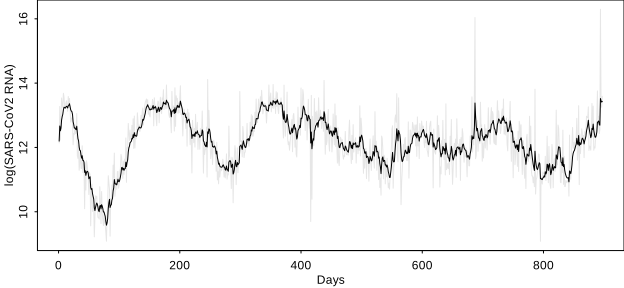
Kalman filtered fit to SARS-CoV2 RNA time series normalized with PMMoV RNA. Data is grey and fit is black.
We see that the filtered fit, shown in Figure 2, is smoother than the data but not as smooth as the fit in Figure 1. Since we believe the state series to be smooth, we could achieve a smoother fit using additional autoregressive terms in the state model for the Kalman filter. We would recommend this in practice, but we have not done it here because we are focussed on the effects of normalization by a control.
| Model | State SD target | State SD control |
State Correlation |
Obs. SD target |
Obs. SD control | Obs Correlation |
Filter SE of state |
|---|---|---|---|---|---|---|---|
| SC2 | 0.136 | 0.522 | 0.249 | ||||
| SC2+PMMoV | 0.133 | 0.025 | 0.088 | 0.523 | 0.410 | 0.231 | 0.246 |
| SC2+BCoV | 0.135 | 0.027 | 0.312 | 0.522 | 0.434 | 0.000 | 0.249 |
From Table 2, we see that the state SD of the target suggests a relative variation from day-to-day of about 14% across all three models. We believe this is higher than the truth and can be reduced by using autoregressive terms. We expect the true level of PMMoV to vary due to sewer effects but the state of BCoV should be constant. We shall show shortly why the estimated state correlation for BCoV should not be interpreted strongly. The observation error SD for the target is similar for the three models and similar to the ad hoc estimate obtained in the previous section. There is a mild correlation between the measurement errors for PMMoV model but practically zero correlation for the BCoV model. We claim that this contrast indicates sewer effects for PMMoV while BCoV reflects only laboratory effects.
The SE of the final filtered state estimate from Table 2 shows only small differences. Using the direct normalization method of the previous section made the variance larger. We have avoided this fate, but we did not achieve much improvement. The adjustment in the filtered estimate due to normalization is about 1%. It is generally an adjustment in the same direction of the direct adjustment of the previous section, but significantly smaller in size. Simulation evidence from the next section suggests we cannot be confident of even this small improvement. The Kalman updating step takes a form analogous to Equation (5) but the size of the step is reduced. Despite the possibility of some bias reduction, the results are disappointing as normalization using the controls has yielded no clear benefit. Under what circumstances might they be more effective?
Simulation
We use simulation to explore the generality of the conclusions from the previous section and discover scenarios where the Kalman filtering normalization is clearly beneficial. We consider four simulated scenarios:
Data generated from the model for SARS-CoV2 and PMMoV RNA with parameters set to those estimated from the observed data in the previous section. We use this to check the stability of our conclusions.
Data generated from the same model except with an observation error correlation of 0.8, much higher than the 0.23 observed. In this scenario, the target and control measurement are more tightly linked.
Data generated from the first model except with a 10 times smaller control variation. In this scenario, the control can be measured with greater precision.
Data generated from the first model except with a much stronger correlation between the states of 0.8 compared to the 0.09 observed. In this scenario, the covariation of the target and control through the sewer are more tightly linked.
In each scenario, we generate 1000 simulated datasets and report the mean estimates in Table 3.
| Model | State SD target | State SD control |
State Correlation |
Obs. SD target |
Obs. SD control | Obs. Correlation |
Filter SE |
|---|---|---|---|---|---|---|---|
| Observed Data | 0.132 | 0.024 | 0.063 | 0.523 | 0.411 | 0.232 | 0.244 |
| High Obs. Correlation | 0.131 | 0.024 | 0.037 | 0.520 | 0.408 | 0.792 | 0.203 |
| Low control SD | 0.137 | 0.026 | 0.087 | 0.519 | 0.128 | 0.236 | 0.244 |
| High State Correlation | 0.135 | 0.023 | 0.723 | 0.519 | 0.410 | 0.235 | 0.245 |
In the case where we simulate from the fitted model, the mean results are close to the fitted estimates indicating a lack of bias in the fitting process. We can also use the simulated values to estimate the uncertainty in the parameter estimates (see supplementary materials for details). Most of the estimates have low enough variation to support our previous conclusions, but the estimate of the state correlation was found to be highly variable indicating that it is difficult to estimate this parameter well. This indicates why the values in Table 2 for this parameter must be viewed with caution.
For the three scenarios where we perturb the parameters, we see that the estimated parameters are obtained without substantial bias. Only in the high observed error correlation situation do we observe worthwhile improvement in the filtered state SD. To realize this improvement, we would need to find a control whose measurement is much more strongly correlated with the target. Given current PCR technology, there is no candidate for such a control.
We have used a simple bivariate Kalman filter in these examples to focus on the issue of variance reduction via a control. We could use autoregressive terms to improve the fit, but this would not improve the value of the controls. The controls could also be introduced as regressors in the model, but the weak correlation would remain an obstacle. We have used a Gaussian Kalman Filter but for targets that appear intermittently or with very low prevalence, we can adapt the method to use other distributions. An example of this can be seen in (Cluzel et al., 2022). The Kalman filter is an example of dynamic linear model with wider applications in WBE found in (Ouyang et al., 2025).
Alternatives for Variance Reduction
We have seen that it is difficult to achieve worthwhile variance reduction by using a control in situations typical of PCR measurement of targets in WBE. There are some alternative avenues for improvement. The high variation in the measurement of the laboratory control BCoV suggests that the PCR measurement is the single largest component in the overall variation of the target measure. One might hope for technical improvements in this technology.
The most used tool for variance reduction is replication. One additional true replicated measurement would reduce the standard error for the mean of the now two measurements by a factor of This would be superior to any improvement seen above, even in the simulated scenarios. There are difficulties with this approach. Replication is already used in WBE – in our example data, at least six replicates were used, although only the mean was reported. Further improvements by using more replications are subject to diminishing returns as the standard error is inversely proportional to the square root of the number of replications. A further difficulty is that a true replicate means repeating the collection and processing steps from the source at the WWTP. A replicate derived from division of the sample at a later stage will be less effective.
Smoothing is related to replication in that recent measurements are combined with the current measurement. Various methods including rolling averages are used. The Kalman filter method described earlier can incorporate autoregressive terms. This is an effective method of variance reduction. Because we can only smooth over a small number of days, the variance reduction is limited.
In (Schenk et al., 2024), RNA measurements for other common pathogens, such as Norovirus or Influenza are available. We can incorporate all these targets into a single Kalman filter model. Since these other targets are subject to many of the same sources of variation, the statistical effect of borrowing strength will occur, improving the estimates and reducing the variation. Another idea is to measure a different gene target for the same RNA.
We may also return to models that use prevalence information of the form seen in Equation (1), but with the requirement that the control or adjusting variables are used in an explicit process model that allows the knowledge of appropriate normalization to be extrapolated to new scenarios with different targets and locations. Perhaps, something like the parameterization of the normalization seen in (Leisman et al., 2024) might be of benefit.
Conclusion
We have shown that using controls to normalize PCR measurements in WBE for the purposes of variance reduction is challenging. Meanwhile, these controls have other uses. A control that reflects variation in the sewer contains useful information about the population in the catchment area of the WWTP. A control which is introduced into the sample after collection is still useful for quality control purposes. Thus, we are not claiming such controls have no value, but researchers should consider whether measuring other pathogen RNA markers is a better use of limited resources. The Kalman filter model used here presents a framework where control and other auxiliary information can be used to potential improve the estimate of the primary target that can be used in online settings as new data becomes available.
Acknowledgements
Funding from the Centre of Excellence in Water-Based Early-Warning Systems for Health Protection (CWBE) at the University of Bath
Conflicts of interest
There are no conflicts of interest
Data and Code Availability
Data and code supplied in the supplementary materials.
References
- Ahmed, T., Philo, S. E., Boehm, A. B., Halden, R. U., Bibby, K., & Delgado Vela, J. (2026). Assessing normalization methods in wastewater based epidemiology: a systematic review. Environmental Science: Water Research & Technology, 12(5), 1374–1382. https://doi.org/10.1039/d5ew01049g
- Boehm, A., Bidwell, A., Wolfe, M., Zulli, A., Duong, D., Shelden, B., & White, B. (2025). Data for Human pathogen nucleic acids in wastewater solids from 191 wastewater treatment plants in the United States [Dataset]. Stanford Digital Repository. https://doi.org/10.25740/HJ801NS5929
- Cluzel, N., Courbariaux, M., Wang, S., Moulin, L., Wurtzer, S., Bertrand, I., Laurent, K., Monfort, P., Gantzer, C., Guyader, S. L., Boni, M., Mouchel, J.-M., Maréchal, V., Nuel, G., & Maday, Y. (2022). A nationwide indicator to smooth and normalize heterogeneous SARS-CoV-2 RNA data in wastewater. Environment International, 158, 106998. https://doi.org/10.1016/j.envint.2021.106998
- Darling, A., Davis, B. C., Byrne, T., Deck, M., Maldonado Rivera, G. E., Price, S., Amaral-Torres, A., Markham, C., Gonzalez, R. A., Vikesland, P. J., Krometis, L.-A. H., Pruden, A., & Cohen, A. (2025). Comparative Assessment of Wastewater-Based Surveillance Normalization Methods to Improve Pathogen Monitoring in Rural Sewersheds. Environmental Science & Technology, 59(22), 11095–11107. https://doi.org/10.1021/acs.est.4c14485
- Deák, G., Lupu, L., & Prangate, R. (2026). A Systematic Review of Methodological Approaches to SARS-CoV-2 Wastewater Surveillance. Viruses, 18(2), 205. https://doi.org/10.3390/v18020205
- Durbin, J., & Koopman, S. J. (2012). Time Series Analysis by State Space Methods. Oxford University Press. https://doi.org/10.1093/acprof:oso/9780199641178.001.0001
- Helske, J. (2017). KFAS: Exponential Family State Space Models in R. Journal of Statistical Software, 78(10). https://doi.org/10.18637/jss.v078.i10
- Lamm, E. D., Babler, K. M., Sharkey, M. E., Amirali, A., Beaver, C., Boone, M. M., Comerford, S., Cooper, D., Currall, B., Grills, G. S., Kobetz, E., Kumar, N., Laine, J., Lamar, W. E., Lyu, J., Kennedy, A., Perritano, S., Mason, C. E., Reding, B. D., … Solo-Gabriele, H. M. (2025). Inclusion of Physical–Chemical Water Quality Measurements Can Improve Associations between SARS-CoV-2 RNA Levels in Wastewater and COVID-19 Cases within Smaller Sewersheds. Journal of Environmental Engineering, 151(9). https://doi.org/10.1061/joeedu.eeeng-8138
- Leisman, K. P., Owen, C., Warns, M. M., Tiwari, A., Bian, G. (Zhixin)., Owens, S. M., Catlett, C., Shrestha, A., Poretsky, R., Packman, A. I., & Mangan, N. M. (2024). A modeling pipeline to relate municipal wastewater surveillance and regional public health data. Water Research, 252, 121178. https://doi.org/10.1016/j.watres.2024.121178
- Marsaglia, G. (2006). Ratios of Normal Variables. Journal of Statistical Software, 16(4). https://doi.org/10.18637/jss.v016.i04
- Ouyang, D., Chung, L., Osborn, M., Schacker, T. W., & Doss, C. R. (2025). Dynamic Linear Models for Wastewater-Based Epidemiology with Missing Values: an Application to Covid-19 Surveillance. Data Science in Science, 4(1). https://doi.org/10.1080/26941899.2025.2562199
- Pellett, C., Farkas, K., Williams, R. C., Wade, M. J., Weightman, A. J., Jameson, E., Cross, G., & Jones, D. L. (2024). Multi-factor normalisation of viral counts from wastewater improves the detection accuracy of viral disease in the community. Environmental Technology & Innovation, 36, 103720. https://doi.org/10.1016/j.eti.2024.103720
- Rosengart, A. L., Bidwell, A. L., Wolfe, M. K., Boehm, A. B., & Townes, F. W. (2025). Spatiotemporal Variability of the Pepper Mild Mottle Virus Biomarker in Wastewater. ACS ES&T Water, 5(1), 341–350. https://doi.org/10.1021/acsestwater.4c00866
- Schenk, H., Rauch, W., Zulli, A., & Boehm, A. B. (2024). SARS-CoV-2 surveillance in US wastewater: Leading indicators and data variability analysis in 2023–2024. PLOS ONE, 19(11), e0313927. https://doi.org/10.1371/journal.pone.0313927
- Sweetapple, C., Wade, M. J., Melville-Shreeve, P., Chen, A. S., Lilley, C., Irving, J., Grimsley, J. M. S., & Bunce, J. T. (2023). Dynamic population normalisation in wastewater-based epidemiology for improved understanding of the SARS-CoV-2 prevalence: a multi-site study. Journal of Water and Health, 21(5), 625–642. https://doi.org/10.2166/wh.2023.318
- Verani, M., Federigi, I., Angori, A., Pagani, A., Marvulli, F., Valentini, C., Atomsa, N. T., Conte, B., & Carducci, A. (2025). Evaluating Population Normalization Methods Using Chemical Data for Wastewater-Based Epidemiology: Insights from a Site-Specific Case Study. Viruses, 17(5), 672. https://doi.org/10.3390/v17050672