Abstract
Entity resolution (also known as record linkage) aims to classify which database items, or file records, refer to the same entity, where the entity is typically a real-world object such as a person, business or product. Transformer models have brought artificial intelligence to text-based entity resolution through their superior ability for natural language processing. However, applying a transformer model directly to “link or not to link” a large number of record pairs can be computationally too costly in practice. We propose a workflow of text-based entity resolution that extends traditional approaches to record linkage by incorporating judicious uses of transformer models. A bi-encoder is used for text embedding and blocking, while traditional generative or discriminative models can be used for scoring and classification. A cross-encoder can then be reserved for selected harder cases, providing a mechanism for trading linkage accuracy against computational cost. We also discuss fine-tuning and provide a workable approach to linkage error assessment for the combined procedure. The proposed workflow is evidenced and illustrated using two benchmark datasets from the Magellan data repository.
1 Introduction
The task of entity resolution is to classify the database items (or file records) that refer to the same entity (Christen, 2012), where the entity may be person, business, product, etc. In this context, any two items corresponding to the same entity are said to form a match, whereas the two items may or may not be classified as a link at the result of entity resolution. The need of entity resolution arises in official statistics, machine learning, research or knowledge synthesis, and many other areas, where it is often the prerequisite of downstream tasks that treat the linked dataset as a single source of input.
Record linkage across two files is a typical problem of entity resolution (e.g. Fellegi & Sunter, 1969; Jaro, 1989; Lee et al., 2022; Newcombe et al., 1959). Instead of hand-crafted rules for link classification, the probabilistic approach asks one to model the distortions of the linkage key variables, or simply keys, such as (name, date-of-birth, address) for records of persons, so that the decision whether or not to link two records can be largely or entirely data-driven (i.e. without the need for clerical review).
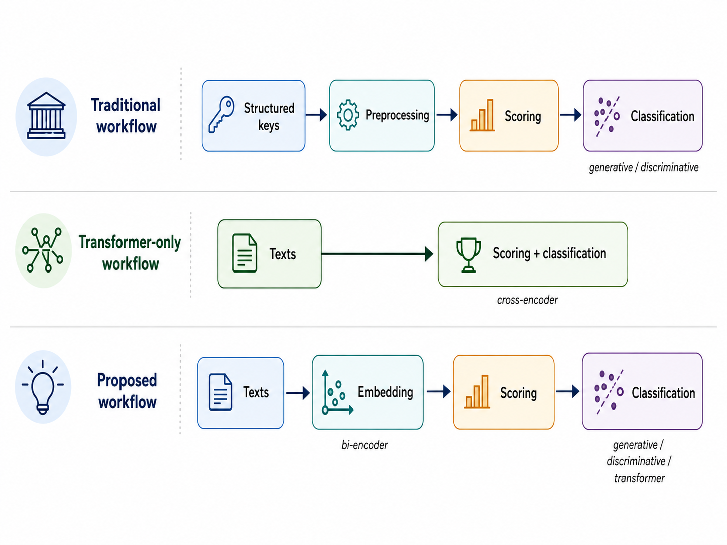
The traditional workflow of probabilistic linkage may be given generically as in Figure 1. Although the key values are given as structured data, preprocessing is often necessary to accommodate typical variations of the same key, such as different spellings of an address or name. Scoring then refers to the statistical modelling of the key-value distortions. Two possibilities may be considered.
Generative models have been common ever since Fellegi & Sunter (1969), where one models the probability of the observed key-value agreement pattern of a pair of records given that they form a match, and the probability given that they do not form a match. The ratio of these two probabilities forms the basis for link classification.
Discriminative models target the probability that a pair of records form a match given their observed key values or key-value agreement pattern. While uncommon for record linkage in the unsupervised setting, these models arise naturally in the supervised setting where labelled matches are available. Logistic regression, which we consider later in this paper, is one such model.
Finally, Fellegi & Sunter (1969) use the likelihood ratio resulting from generative models to classify links and non-links directly, leaving a subset of record pairs to be decided by clerical review. Lee et al. (2022) propose maximum entropy classification (MEC) for record linkage based on generative models, which enables fully automated link classification guided by the estimated rates of false links and missing matches.
| Field | DBLP-Scholar text |
|---|---|
| Title | Distributed Representations of Tuples for Entity Resolution |
| Author | Z Ebraheem, Thirumuruganathan, S. Joty |
| Venue | Proc. VLDB Endow. |
| Year | 2018 |
| Field | Abt-Buy text |
| Name | Sony Black Pocket AM/FM Walkman Radio - SRF59 |
| Description | Belt Clip Included / Uses 1 AA Battery / Local/DX Switch... |
However, for entity resolution based on messy texts instead of structured key values, it is often difficult and ineffective to formulate deterministic rules of preprocessing. Table 1 gives two examples, one from the DBLP-Scholar dataset and the other from the Abt-Buy dataset, both in the Magellan data repository of benchmark datasets for entity resolution (Konda et al., 2016); see Appendix A for details.
The text data in DBLP-Scholar are structured in four fields. Although the content can be quite noisy for some fields, such as author names, one might still attempt preprocessing of these texts by hand-crafted rules. In contrast, the relatively free-form texts in the Abt-Buy dataset may be highly irregular from one product to another, and it is not obvious that traditional preprocessing rules for keys such as name and address would be effective for the product names and descriptions here.
It is therefore natural to consider machine learning models that can work directly with such text. Mudgal et al. (2018) show that deep-learning models can outperform hand-crafted feature engineering for text-based entity resolution. More recently, transformer models, introduced by Vaswani et al. (2017), have provided a way to represent and compare texts while taking their context into account. The transformer architecture uses self-attention to model relationships between tokens within a sequence, which makes it particularly suitable for handling textual data.
In the work of Li et al. (2020), entity resolution is cast as a sequence-pair classification task using a pretrained transformer language model. The two records are supplied jointly to the model, allowing the self-attention layers to represent interactions across the paired input. This type of architecture is commonly referred to as a cross-encoder.
The computational cost becomes prohibitive, however, if the cross-encoder is applied to every possible pair of records, as we shall illustrate later using the DBLP-Scholar and Abt-Buy datasets. A bi-encoder transformer model (Reimers & Gurevych, 2019; R. Wang et al., 2023) instead encodes each text separately as a numerical vector, or embedding. Similarity between these embeddings can then be used to identify a much smaller set of candidate records before more expensive scoring or classification is applied. This provides a form of semantic blocking, analogous to traditional blocking in record linkage. For instance, Reimers & Gurevych (2019) report that finding the most similar pair in a collection of sentences required about 65 hours with a standard BERT model, compared with about 5 seconds using SBERT embeddings and cosine similarity.
Bi-encoder blocking greatly reduces the number of record pairs that require further comparison, but it still leaves several choices about how the candidate pairs should be scored and classified. In particular, the numerical representations produced by a bi-encoder can be combined with traditional generative or discriminative scoring methods, or the candidate texts can be passed to a cross-encoder for classification. The usefulness of these alternatives may also change after the transformer models are fine-tuned to the texts of a particular application. These considerations motivate the integrated workflow in Figure 1, as well as a closer examination of the linkage errors associated with the resulting models.
1.1 Proposed workflow using transformer models
Our proposed workflow for entity resolution is given in Figure 1, which uses transformer models as well as traditional generative or discriminative models.
While the workflow is applicable to both the supervised and unsupervised settings, i.e. with or without a sample of labelled matches, we shall focus on the supervised setting in this paper. Transformer models are considered for embedding and classification. Notice that cross-encoder models with text as input are not relevant for scoring given numerical embeddings, whereas how to use transformer models to achieve scoring-classification from texts directly remains an open question in the unsupervised setting.
A fundamental difficulty for modelling arises from the following fact about entity resolution. While matched items refer to real entities, a pair of non-matches does not correspond to a single real entity. For instance, when two records refer to two different persons, there is no person associated with both records. It follows that there is no naturally defined population of non-matches corresponding to the population of matches, which complicates the construction of training data for supervised learning.
To deal with this difficulty, it is common to create the training and test sets in a way that mirrors how the models will later be applied to out-of-sample items. Suppose that, for each out-of-sample record in , one would conduct blocking to gather candidate records in for scoring and classification. We then construct candidate records in the same manner for the sampled file- records, and partition those file- records into training and test sets together with their associated candidate records. Thus, all candidate pairs associated with a given file- record remain in the same partition. Duplication of candidate records for different records in is allowed if it is also allowed for the out-of-sample records in application.
Notice that, if none of the valid matched records is selected among the candidates, the corresponding file- record cannot be linked correctly. Hence the choice of induces a floor of missing match rate (MMR). In practice, for scoring and classification, it is natural to select the most likely link candidates for blocking, i.e. the records in with the most similar texts, and to choose such that the MMR floor is considered acceptable. Selecting the most similar candidates also provides more difficult non-matches for supervised learning than selecting non-matches randomly.
In addition to the MMR, another central performance measure is the false linkage rate (FLR). We use the FLR and MMR, following the definitions of Lee et al. (2022), for the evaluation and comparison of the different methods considered in this paper. Their formal definitions in the present setup are given in Section 1.3. Notice that both are well-defined whether or not one employs additional treatments of duplicated candidate records for scoring and classification.
The details of the steps in the proposed workflow will be studied in this paper, and the relevant methodological choices exemplified and compared.
1.2 Link classification errors by transformer models
The estimation of FLR and MMR for link classification based on transformer models requires special attention.
If one uses only a pretrained transformer model that is fixed independently of the labelled data, then, under the SRSWOR assumption stated in Section 1.3, the observed errors in the labelled file- sample may be used to estimate the FLR and MMR that would arise over the corresponding finite population of file- records.
The matter becomes more complicated when the transformer model is fine-tuned using the labelled sample. An obvious approach is to split the labelled sample into a training set for fine-tuning and a test set for estimating the errors of the resulting subsample-tuned model. This is valid if one is willing to apply that subsample-tuned model directly to the out-of-sample items. It is not sufficient, however, if the subsample training is used only to determine the hyperparameters of fine-tuning, after which the transformer model is fine-tuned again using the entire labelled sample and this final model is applied to the remaining records. The errors observed on the original test set then refer to a different fitted model from the one eventually used for entity resolution.
We shall study this issue later using the DBLP-Scholar and Abt-Buy datasets, illustrating both the statistical problem and the practical difficulties that arise. Below we briefly explain why the issue also presents difficulties for several existing approaches to error assessment.
Bayesian uncertainty propagation. In Bayesian approaches to entity resolution, one may model the key values or their disagreement patterns and generate link sets according to the posterior distribution of the matches, conditional on the observed keys; see, for example, Tancredi & Liseo (2011); Sadinle (2017); Steorts et al. (2016). It is unclear how such prior-posterior uncertainty propagation can be carried through a fine-tuned transformer model, which does not provide the likelihood function required for the corresponding Bayesian calculation. Moreover, repeatedly generating link sets while refitting or evaluating a large transformer model would be computationally expensive.
Auditing. A practical approach in the unsupervised setting of entity resolution is to draw an audit sample from the classified links in order to estimate the FLR (Christen, 2012); see also Binette et al. (2024) for a more elaborate proposal. In the supervised setting, the labelled match sample can be used to estimate both FLR and MMR when the classification model is fixed independently of that sample. The situation changes when the same labelled observations are used for fine-tuning. Auditing additional out-of-sample records could provide information about the final model, but identifying their true matches may require substantial clerical effort.
Design-based sample inference. Zhang et al. (2025, 2026) develop unbiased estimation of algorithmic prediction or classification errors under finite population sampling. In principle, this provides a way to accommodate models trained using sampled observations. In practice, however, the required calculations can be costly for transformer models. Moreover, although link classification can be viewed as a special case of classification, unbiased estimation of classification errors in this framework relies on randomised prediction or classification, whereas deterministic classification is generally preferred for record linkage.
1.3 Notations and rest of paper
Let us now introduce the basic notations related to the workflow of entity resolution, formalising the concepts discussed above and preparing for the investigations later.
Without loss of generality, let us use the standard setup of record linkage across two files. Let and be two files containing and records, respectively. Let entity resolution, or record linkage, be based on , where is the text associated with record , which may or may not consist of structured fields, as exemplified in Table 1.
Let be the set of matches, , and denote a match by , or equivalently , if records and refer to the same entity. A non-match is denoted by , or . Let and denote the records in and , respectively, belonging to .
Let denote the sampled file- records. For simplicity of exposition in this paper, we assume that is obtained from by simple random sampling without replacement (SRSWOR). Let
denote the labelled match relation induced by these sampled records. Let denote the records in having at least one match in , and let denote the corresponding matched records in . Thus, contains the sampled file- records that are non-matchable.
In practice, one first draws the file- records in and then identifies all their known matches by any means necessary. This formulation samples file- records rather than individual matched pairs. The distinction becomes relevant when a file- record has more than one valid partner in .
To limit the number of comparisons for the models, let denote the block of candidate records for each according to a given blocking scheme, where , and may be non-empty for . Let be the size of in the case .
By applying a given model of link classification to denote by if is linked and if it is not linked. One can estimate the FLR and MMR when the model is applied to all the record pairs as where refers to the linked record in given , and if .
For supervised learning including non-matches in addition to matches, let denote a partition of , where
We use for training and for testing. Let
denote the labelled match relations induced by these two sets of file- records. Thus, all known matches belonging to the same file- record remain on the same side of the training-test partition.
According to the setup in Section 1.1, the corresponding candidate non-matches associated with matchable records are
for training and
for testing. For non-matchable sampled file- records, all candidate pairs are non-matches, giving
Notice that the setup of supervised learning above can vary with the blocking scheme. In particular, given the fixed block size , we consider two schemes.
-
Scheme-I: for each , let contain one retained matched record for which , together with non-matches.
-
Scheme-II: for each , let consist of the most similar file- records.
Under Scheme-I, the retained labelled match is inserted into each candidate block, whereas under Scheme-II the candidate block is determined entirely by similarity and may therefore fail to contain a valid match. The difference between the two schemes decreases as the block size increases. Scheme-I makes more efficient use of the labelled matches for learning, while Scheme-II is more closely related to the application of the models to out-of-sample records.
In the experiments below we use Scheme-II to construct the candidate blocks. For supervised fitting, however, one known valid file- partner is retained as the positive example for each matchable file- record, whether or not that particular retained partner occurs in . The non-match examples are drawn from , with every known valid partner excluded from the non-match class. At evaluation, is not augmented in this way: a predicted link must be selected from the retrieved candidate block, and failure to retrieve any valid partner contributes to the floor MMR.
Section 2 describes the datasets and experimental setup used throughout the empirical analysis. We study the proposed workflow using pretrained transformer models in Section 3. Section 4 considers the fine-tuning of transformer models, including the related assessment of link classification errors. Section 5 provides the final remarks and discusses topics for future research and development.
2 Data and experimental setup
2.1 Datasets and preprocessing
We use the DBLP-Scholar and Abt-Buy datasets from the Magellan repository (Konda et al., 2016). The two datasets differ considerably in both scale and the form of their textual information. DBLP-Scholar contains bibliographic records, whereas Abt-Buy contains product records collected from two online retailers. Our evaluation reformulates these benchmark datasets as record-level candidate retrieval and linkage problems, with FLR and MMR calculated over file- records and their candidate sets. These error rates are therefore not directly comparable to the pair-level precision, recall or F1 scores reported under the standard entity-matching classification protocol in, for example, DeepMatcher and Ditto (Li et al., 2020; Mudgal et al., 2018). Table 2 summarises the data used in the experiments.
| Dataset | Gold pairs | Matchable records in | ||
|---|---|---|---|---|
| DBLP-Scholar | 2,616 | 64,263 | 5,347 | 2,408 |
| Abt-Buy | 1,081 | 1,092 | 1,097 | 1,081 |
For DBLP-Scholar, file is the DBLP file and file is the Scholar file. The original files contain the fields title, authors, venue and year. The gold-standard mapping contains 5,347 pairs involving 2,408 distinct DBLP records and 5,218 distinct Scholar records. A DBLP record may therefore have more than one valid Scholar partner. Of the 2,616 DBLP records, 2,408 have at least one gold-standard match.
For Abt-Buy, file is the Abt file and file is the Buy file. The original Abt file contains the product name, description and price, while the Buy file additionally contains the manufacturer. The gold-standard mapping contains 1,097 pairs. All 1,081 Abt records have at least one known match in the Buy file, and some records have more than one valid partner.
For semantic blocking, we use the title field for DBLP-Scholar and the product-name field for Abt-Buy. These fields contain no missing values in either dataset. The other common text fields remain available for the field-level comparisons used by the traditional scoring models. The complete gold-standard mappings are retained when determining whether a candidate set contains a valid match and when evaluating a predicted link.
For constructing supervised match examples, one valid file- partner is retained for each matchable file- record. Thus, there are 2,408 retained positive pairs for DBLP-Scholar and 1,081 for Abt-Buy. Importantly, the other known valid partners are not treated as non-matches. At evaluation, a predicted link is considered correct if the selected file- record is any known valid partner of the corresponding file- record.
2.2 Training and candidate construction
The experimental unit is a file- record together with its candidate file- records, rather than an individual candidate pair. This distinction is important because all the pairs associated with a given file- record must remain together when the data are divided into training and test sets.
For the main experiments, the file- records are randomly divided 50–50 into training and test sets. In DBLP-Scholar this gives 1,308 records in each half. In Abt-Buy, 540 records are assigned to training and 541 to testing. The primary results reported in Sections 3 and 4 use random seeds 42, 43 and 44 and are averaged over the three resulting splits. In Tables 5–8, numbers in parentheses are Monte Carlo standard errors, calculated as the sample standard deviation of the three seed-level error rates divided by . The FLR and MMR are calculated separately for each split before averaging. With only three replications, these standard errors describe observed split-to-split variation and do not support precise interpretation of small method differences. Seeds 45–51 are used later where additional Monte Carlo replications are required.
Candidate blocks are constructed according to Scheme-II in Section 1.3. First, the pretrained bi-encoder all-MiniLM-L6-v2 is used to embed the blocking text of every record in files and . For each record , the records in are ranked by cosine similarity of their embeddings, and the most similar records form . We consider primarily and , while is also useful for examining the blocking floor.
The same procedure is applied independently to every file- record. Consequently, the same file- record may occur in the candidate blocks of several file- records. This mirrors how semantic blocking would be applied to records outside the labelled sample and avoids imposing an artificial one-to-one restriction at the blocking stage.
The labelled candidate pairs are then constructed for supervised learning. Each retained valid partner provides one positive example for its matchable file- record. This retained positive is supplied for supervised fitting whether or not that particular partner occurs among the retrieved top- candidates. The non-match examples are drawn from the retrieved candidate block: candidate-derived pairs that are not known valid partners are treated as negatives, while every additional gold-standard partner of the same file- record is excluded from the non-match class. Thus, one retained positive may be accompanied by several retrieved hard non-matches rather than by only one negative example. At evaluation, the candidate block is not augmented with the retained positive, so a record cannot be linked correctly when none of its valid partners has been retrieved. The resulting non-matches are therefore relatively difficult examples selected by semantic similarity rather than arbitrary pairs drawn from .
For DBLP-Scholar, the training and test sets also contain file- records that have no gold-standard partner. Their candidate pairs are all non-matches. This is useful because such records occur in the application of record linkage and a classification procedure should be able to leave them unlinked. For Abt-Buy, every file- record has at least one known valid partner.
For discriminative link classification, the candidate pairs belonging to the training half are further divided 80–20 into fitting and validation parts. The fitting part is used to estimate the model and the validation part to choose the link-classification threshold by maximising the F1 score. The outer test records are not involved in this choice.
2.3 Models and implementation
We consider three ways of progressing from the candidate pairs to link classification, corresponding to the workflows introduced in Figure 1.
In the traditional workflow, field-level text comparisons are obtained with the Jaro–Winkler metric. In the proposed workflow, these are replaced by cosine similarities calculated from bi-encoder embeddings. Unless otherwise stated, the bi-encoder is all-MiniLM-L6-v2 (Reimers & Gurevych, 2019). Section 3.1 explains how these comparison outcomes enter the subsequent scoring models.
Two traditional scoring models are used in the main comparison. The generative model follows the MEC approach of Lee et al. (2022), with the match and non-match densities of the continuous comparison outcomes estimated by kernel density estimation. For every MEC fit, the per-field match and non-match densities are estimated with sklearn.neighbors.KernelDensity using a fixed bandwidth of 0.05. The bandwidth is held fixed across fields, datasets, random splits and block sizes rather than reselected from the data. The discriminative model is logistic regression. A radial-kernel SVM, XGBoost and a small multilayer perceptron are considered later as a sensitivity analysis.
For direct classification from paired texts, we use the cross-encoder ms-marco-MiniLM-L-6-v2. Both transformer models are first considered in their pretrained form. Their fine-tuning is then investigated in Section 4.1, where we give the corresponding training settings and explain how the candidate blocks are treated before and after fine-tuning.
The model inputs are constructed as follows. All text fields are lower-cased and stripped of leading and trailing whitespace, with missing values represented by empty strings. For DBLP-Scholar, the fields are used in the order title, authors, venue and year. For Abt-Buy, the fields are product name followed by description; price and manufacturer are not used. For cross-encoder classification, the fields of each record are concatenated in this order with the literal separator [SEP] , and the two resulting record strings are supplied as the paired input to the cross-encoder. The tokenizer then applies the configured maximum sequence length of 128 tokens. For bi-encoder scoring, by contrast, each field is encoded separately with all-MiniLM-L6-v2, and the comparison vector for a candidate pair consists of the fieldwise cosine similarities in the same order. Semantic blocking uses only the title embedding for DBLP-Scholar and the product-name embedding for Abt-Buy. During bi-encoder fine-tuning, each training record is serialised using the same full-record field order and [SEP] separator; after fine-tuning, however, all records are re-embedded field by field for blocking and cosine scoring.
For discriminative models, including the cross-encoder, a validation subset of the training pairs is used to choose the threshold for declaring a link by maximising the F1 score. The particular classification rules are described together with the corresponding models below, since they form part of the methodological comparison rather than merely an implementation detail.
The objective of these experiments is not to identify the best possible model or hyperparameter configuration for either benchmark dataset. Rather, the common setup enables us to examine how embedding, scoring, classification and fine-tuning can be combined within the proposed workflow. Accordingly, the reported error rates are intended to illustrate the behaviour of this workflow under a common experimental setup, rather than to establish state-of-the-art entity-matching performance or a benchmark ranking against published systems such as DeepMatcher (Mudgal et al., 2018), Ditto (Li et al., 2020), or the method of Peeters & Bizer (2021).
2.4 Evaluation
The unit of link classification is again a file- record. Given the candidate block , a scoring model ranks or scores its candidate file- records. If a link is declared, let denote the selected record. For models that use a classification threshold, no link is declared when the best candidate does not satisfy that threshold. The generative MEC calculations considered below instead select the highest-ranked candidate according to the estimated density ratio.
A declared link is counted as correct whenever is one of the known gold-standard pairs for record . This is important for both datasets because the gold-standard relation need not be one-to-one. Selecting a valid partner other than the particular partner retained for supervised fitting is therefore still a correct link.
The two error measures are the FLR and MMR defined in Equation (1). It is useful to state their empirical calculation explicitly. Let be the number of links declared among the test file- records, let be the number of those declarations that select a valid gold-standard partner, and let be the number of matchable file- records in the test set. Then
Thus, an incorrect declared link contributes to both error measures: it is a false link among the declarations and, for a matchable file- record, it also means that the true match has not been recovered. An undeclared matchable record contributes to the MMR but not to the numerator or denominator of the FLR. For DBLP-Scholar, a declared link for a non-matchable file- record is necessarily a false link and therefore contributes to the FLR.
Blocking imposes an additional lower bound on the MMR. If none of the valid partners of a matchable file- record occurs in , no scoring or classification model operating on that block can link the record correctly. We refer to the proportion of such records as the floor MMR and examine it explicitly in Section 3.1.
Unless otherwise stated, the tables in Sections 3 and 4 report the mean FLR and MMR over the three primary random splits. In the later investigation of training-set fractions and subsample error assessment, seeds 42–51 provide ten Monte Carlo replications. There we additionally report Monte Carlo standard errors, and, where relevant, relative Monte Carlo standard errors, in order to distinguish variation across random splits from the differences between modelling procedures.
The replication counts were not selected to attain a prespecified hypothesis-testing power or precision target. They reflect the computational cost of repeated fine-tuning and the descriptive purpose of the experiments. Accordingly, the three-split comparisons in Tables 5–8 are used to identify broad patterns rather than to resolve small numerical differences; their Monte Carlo standard errors are reported to show the scale of split-to-split variation. The ten-replication studies in Section 4.3 provide a more precise assessment of training-fraction sensitivity and subsample error estimation, but they are likewise interpreted cautiously when the Monte Carlo standard error is of the same order as the observed difference or bias.
3 Workflow with pretrained transformer models
The three workflows in Figure 1 handle the text data differently.
In the traditional workflow, the result of text preprocessing would enable one to calculate a similarity measure of any given record pair with associated texts . The Jaro–Winkler metric (Jaro, 1989; Winkler, 1990) is very common in practice, which yields a value between 0 and 1 if appropriately configured. It captures the lexical overlaps, where each text is treated as a string of characters, but is not effective for expressions that differ only superficially to the human eyes, such as “Conf. Proc.” and “Proceedings”.
In the proposed workflow, preprocessing is replaced by embedding, which uses a bi-encoder model to turn each given text into a numerical vector, denoted by , which typically has a dimension of hundreds or more. A common similarity measure of is the cosine similarity of , given as
The bi-encoder similarity measure can capture semantic similarity that is not represented by character-level overlap, while the embeddings can be calculated efficiently and used routinely for the semantic blocking needed before scoring-classification.
In the workflow using a cross-encoder model, which takes a pair of texts and as input directly, one can obtain a score for the similarity between them. A cross-encoder can represent pair-specific interactions between the two texts that similarity measures calculated from separate embeddings, such as above, cannot represent directly. Using a bi-encoder for semantic blocking, and applying a cross-encoder to the candidate-paired texts can potentially achieve the best link classification performance.
Table 3 illustrates the differences with two citations of Silverman’s 1986 monograph. The Jaro–Winkler metric is only calculated for comparisons per field. The pretrained bi-encoder model all-MiniLM-L6-v2 (Reimers & Gurevych, 2019) yields 384-dimensional embeddings, which result in the cosine similarity measures here. The pretrained cross-encoder model ms-marco-MiniLM-L-6-v2 (W. Wang et al., 2020) yields scores from paired texts directly without numerical embeddings being compared afterwards.
| Text | Jaro–Winkler metric | Bi-encoder cosine | Cross-encoder score |
|---|---|---|---|
| Author | 0.510 | 0.784 | 0.974 |
| Title | 0.856 | 0.872 | 0.991 |
| Venue | 0.933 | 0.969 | 0.999 |
| Year | 1.000 | 1.000 | 0.999 |
| Full citation | – | 0.887 | 0.999 |
All methods rank the field agreements in the same order, from the lowest on author name to the highest on year. However, the numerical values produced by the three methods should not be compared as if they were measured on a common scale: the Jaro–Winkler metric, cosine similarity and cross-encoder output arise from different scoring rules. The example instead illustrates the difference in representation. The cross-encoder evaluates the two names jointly, whereas the bi-encoder must commit “Silverman, B. W.” to a fixed vector without the sight of “Bernard W. Silverman”, and vice versa. Joint encoding allows pair-specific interactions to be represented directly, which separate embeddings cannot do. Whether this architectural advantage translates into lower linkage error is assessed below using the FLR and MMR.
Notice that, for deterministic record linkage, one can already apply a chosen threshold to any of the similarity measures for link classification directly. The cross-encoder has greater flexibility for representing pair-specific interactions, but the computation cost of applying it may be too high for many applications of entity resolution even with bi-encoder blocking. Below we first consider how the proposed workflow of probabilistic linkage allows one to incorporate the traditional models for scoring-classification, so as to reduce the computational cost, albeit without fine-tuning of the transformer models; the workflow with fine-tuning of transformer models will be considered in Section 4 later.
3.1 Embedding and scoring
For scoring by generative or discriminative models, one needs numerical representation of key-value comparisons, denoted by for each field of and , where . The Jaro–Winkler metric is a possibility for the traditional workflow, whereas one can use the cosine similarity measure of bi-encoder embeddings for the proposed workflow.
By the MEC approach using generative models, one would obtain an estimated density ratio for the record pair , which is given as
The product form in Equation (3) assumes that the field-level comparison outcomes are conditionally independent given the match status . This assumption may be violated for related bibliographic fields, such as title, authors and venue. In that case, the product of the field-specific density ratios need not equal the likelihood ratio based on their joint distribution.
Notice that discrete comparison outcomes, i.e. agreement or not, are common for record linkage traditionally, in which case one would replace the density ratio by a probability ratio. Given continuous comparison outcomes , we simply apply kernel density estimation (Silverman, 1986) to estimate the two densities in Equation (3), separately, in the training set of matches and non-matches that are constructed as described in Section 2.2.
Meanwhile, discriminative models target the probability of match given the key-value comparison outcomes, denoted by
We use logistic regression as a basic discriminative model. Other models are possible, such as support vector machine (SVM), gradient-boosted trees (XGBoost) and multilayer perceptron (MLP) neural network. A given discriminative model can be estimated from the training set of matches and non-matches as a single dataset.
Using the labelled records in the DBLP-Scholar and Abt-Buy datasets, we consider blocking scheme-II (Section 1.3) with fixed size for each record in . This induces a floor MMR, since a file- record cannot be linked correctly when none of its valid matched records is included in the candidate block.
| Dataset | Floor-zero | |||
|---|---|---|---|---|
| DBLP-Scholar | 0.022 | 0.006 | 0.001 | 4535 |
| Abt-Buy | 0.278 | 0.082 | 0.003 | 748 |
Table 4 shows the floor MMR for the two datasets, where the candidates for each record in are selected from based on the bi-encoder cosine similarity. At , it is 0.022 for the former and 0.278 for the latter, which means that about 97.8% of the matchable file- records have a valid match as the top candidate in the DBLP-Scholar dataset, whereas about 72.2% do so in the Abt-Buy dataset. This indicates that entity resolution is more difficult in the latter case.
Meanwhile, both the floor MMRs become practically acceptable once is increased to 50, especially because one would have to set to remove the floor (i.e. making the floor MMR zero) for the DBLP-Scholar dataset, or for the Abt-Buy dataset. Because blocking uses only the title field for DBLP-Scholar and the product-name field for Abt-Buy, these floor MMRs also reflect that single-field retrieval design. Incorporating additional fields, such as the product description in Abt-Buy, could potentially lower the blocking floor, but multi-field blocking is not evaluated in the present study.
3.2 Comparison of embedding and scoring methods
The comparison outcomes are calculated for the candidate pairs constructed as described in Section 2.2, either as the Jaro–Winkler metric or the cosine similarity of bi-encoder embeddings. Given , we compare the resulting link classification errors under generative and discriminative scoring models. The FLR and MMR are calculated on the held-out file- records according to Section 2.4.
The distinction between the two scoring approaches is worth explaining. For MEC under the generative model, we link each file- record to the candidate with the highest density ratio in Equation (3). Thus, the best available candidate is always selected. For a discriminative model one could similarly select the candidate with the highest match probability in Equation (4). However, this would force a link even when all the candidate probabilities are small.
We therefore consider a threshold-based classification rule for the discriminative models. As described in Section 2.2, a validation subset of the training pairs is used to choose the threshold that maximises the F1 score. A link is declared only when the highest-scoring candidate exceeds this threshold; otherwise the file- record is left unlinked. This provides a useful contrast with the generative procedure because it allows the model to abstain when the candidate evidence is weak. We do not investigate alternative cross-validation schemes or decision criteria here, since our purpose is to illustrate the role of discriminative scoring-classification within the proposed workflow rather than to optimise the procedure for these two datasets.
| Key-value comparison | Scoring-classification | FLR | MMR | FLR | MMR |
| String, Jaro–Winkler | Generative, kernel density | 0.034 (0.0026) | 0.018 (0.0005) | 0.046 (0.0031) | 0.013 (0.0002) |
| Discriminative, logistic | 0.030 (0.0038) | 0.036 (0.0030) | 0.027 (0.0027) | 0.050 (0.0034) | |
| Bi-encoder, cosine | Generative, kernel density | 0.023 (0.0013) | 0.018 (0.0015) | 0.043 (0.0026) | 0.014 (0.0009) |
| Discriminative, logistic | 0.016 (0.0038) | 0.056 (0.0028) | 0.009 (0.0027) | 0.068 (0.0027) | |
| String, Jaro–Winkler | Generative, kernel density | 0.389 (0.0089) | 0.500 (0.0043) | 0.449 (0.0097) | 0.525 (0.0075) |
| Discriminative, logistic | 0.343 (0.0279) | 0.597 (0.0385) | 0.338 (0.0081) | 0.662 (0.0468) | |
| Bi-encoder, cosine | Generative, kernel density | 0.278 (0.0044) | 0.425 (0.0062) | 0.327 (0.0043) | 0.356 (0.0073) |
| Discriminative, logistic | 0.248 (0.0191) | 0.479 (0.0505) | 0.233 (0.0210) | 0.543 (0.0597) | |
Table 5 reports the test set FLR and MMR for four combinations of embedding and scoring methods, given two block sizes . The results are averaged over three random 50–50 training-test splits, with Monte Carlo standard errors in parentheses. Comparisons of close means should be read in light of this split-to-split variation.
Regarding bi-encoder embeddings instead of the traditional character-string comparisons, the effects are not obvious for the DBLP-Scholar dataset where the texts are less messy (Table 1). The bi-encoder yields lower FLRs in all four comparisons, but does not consistently reduce the MMR. In contrast, the improvements are clearly visible for the Abt-Buy dataset with more messy texts. Both the FLR and MMR are reduced by the bi-encoder representation for either scoring model and either block size.
These results illustrate the potential advantages of transformer-based embeddings for text-based entity resolution. Notice that the performance of the bi-encoder can be further changed by fine-tuning, which will be considered in Section 4.
Regarding scoring-classification by generative or discriminative models, the results here show that the discriminative logistic regression model yields lower FLRs than the generative kernel density model, whereas the latter yields lower MMRs. The distinction is especially clear for the Abt-Buy dataset. This reflects the different link-classification rules used here: we always link the top-ranked candidate under the generative model, whereas a validation split is used to determine a threshold for the discriminative model, which may abstain from declaring a link. Accordingly, the FLR/MMR contrast in Table 5 should not be interpreted as an intrinsic difference between generative and discriminative model families; it also reflects the different decision rules applied to their scores.
Without advocating for one modelling approach against the other generally, we note that scoring-classification by discriminative models is worth considering in practice, although such models have been less common in record linkage traditionally.
For completeness, we also apply the pretrained cross-encoder directly to the candidate pairs obtained from bi-encoder blocking. Since the cross-encoder operates on paired record texts rather than on the numerical comparison outcomes used by the traditional scoring models, we report its results together with those of the fine-tuned cross-encoder in Table 7. This allows the effect of task-specific fine-tuning to be assessed separately from that of using the cross-encoder architecture itself.
Regarding the proposed workflow, using the bi-encoder model for embedding and the traditional generative or discriminative models for automated scoring-classification can reduce the number of candidate pairs that need to be processed by a cross-encoder, compared with applying the cross-encoder to every candidate block. This provides the basis for examining the accuracy-cost tradeoff after fine-tuning, compared with either the traditional workflow without transformer models or the transformer-only workflow.
3.3 Sensitivity analysis
Here we conduct sensitivity analysis of a methodological choice not covered above, which exemplifies the relevant considerations in practice and helps to prepare the ground for fine-tuning transformer models later.
| Dataset | Model | FLR | MMR | FLR | MMR |
| DBLP-Scholar | Logistic | 0.016 (0.0038) | 0.056 (0.0028) | 0.009 (0.0027) | 0.068 (0.0027) |
| SVM | 0.017 (0.0021) | 0.040 (0.0037) | 0.018 (0.0017) | 0.041 (0.0048) | |
| XGB | 0.033 (0.0030) | 0.021 (0.0014) | 0.024 (0.0055) | 0.041 (0.0050) | |
| MLP | 0.030 (0.0025) | 0.030 (0.0016) | 0.026 (0.0024) | 0.034 (0.0066) | |
| Abt-Buy | Logistic | 0.248 (0.0191) | 0.479 (0.0505) | 0.233 (0.0210) | 0.543 (0.0597) |
| SVM | 0.252 (0.0170) | 0.592 (0.0274) | 0.211 (0.0235) | 0.701 (0.0348) | |
| XGB | 0.399 (0.0096) | 0.538 (0.0187) | 0.296 (0.0130) | 0.551 (0.0235) | |
| MLP | 0.251 (0.0111) | 0.438 (0.0238) | 0.228 (0.0202) | 0.565 (0.0704) | |
Instead of logistic regression, one can use many other discriminative models. Table 6 compares it to a radial-kernel SVM, an XGBoost and a small MLP net, all based on the same bi-encoder embeddings. The SVM is fitted with an RBF kernel and probability estimation enabled; XGBoost uses 200 trees, maximum depth 4, learning rate 0.1 and log-loss as the evaluation metric; and the MLP has hidden layers of sizes 64 and 32 and a maximum of 300 iterations. The random-split seed is passed to each classifier, and otherwise the defaults of the pinned library versions are used. The FLR and MMR are obtained in the same way as above, and the results of logistic regression are reproduced from Table 5 for easy comparison. The models exhibit different tradeoffs between the two error measures. For DBLP-Scholar, logistic regression has low FLR in both block-size configurations, while several models have lower observed MMR. The FLR estimates for logistic regression and SVM at are close relative to their Monte Carlo standard errors. For Abt-Buy, the FLR and MMR comparisons vary with the model and block size, with appreciable split-to-split variation in several entries. For XGBoost on Abt-Buy, the validation-selected decision threshold lies near 0.45 on the 0.05 grid, so small numerical differences in the embeddings, such as those between CPU and GPU computation, can move it by one grid point and shift the FLR and MMR in opposite directions by more than 0.01. Logistic regression provides a simple discriminative model and will be used as the default for the investigation later.
4 Workflow with fine-tuning of transformer models
Fine-tuning of pretrained transformer models can be important for the application at hand. In the proposed flow of entity resolution, this concerns the bi-encoder model for embedding and the cross-encoder model for direct text-to-link classification.
4.1 Fine-tuning transformer models
Using the training-test construction described in Section 2.2, we now consider task-specific fine-tuning of the bi-encoder and cross-encoder models. The same random splits and treatment of multiple valid partners are retained, so that the results can be compared directly with those obtained using the pretrained models.
There is one important distinction between the two fine-tuning experiments. After fine-tuning the bi-encoder, the records are re-embedded and the candidate blocks are reconstructed from the fine-tuned embeddings before the traditional scoring models are evaluated. For the cross-encoder, the candidate blocks obtained from the pretrained bi-encoder are held fixed. Thus, the cross-encoder comparison isolates the effect of fine-tuning the classifier rather than changing the candidate set at the same time.
The hyperparameters for learning transformer models involve at least four choices: the warmup step, typically set to around 10%; the learning rate, typically of the order ; the number of epochs, typically small; and the batch size, typically 16 or 32. While some experimentation is needed to settle the hyperparameters in practice, it is rare to apply cross-validation inside the training set formally due to the computation cost this would require. Notice that the computation cost differs for bi-encoder and cross-encoder. Once the embeddings from a bi-encoder have been obtained, similarity calculation and subsequent scoring are computationally cheap. In contrast, the cross-encoder must process each pair of texts directly whenever it is applied.
The bi-encoder model all-MiniLM-L6-v2 is trained for one epoch with ContrastiveLoss, using 10% linear warmup, batch size 16 and learning rate . The contrastive loss encourages the embeddings of matched record pairs to be closer and those of non-matched pairs to be further apart. The fine-tuned bi-encoder model can then be applied to the records in to yield the fine-tuned embeddings, from which the per-field cosine similarities are calculated as before.
The cross-encoder ms-marco-MiniLM-L-6-v2 is trained for five epochs with 10% linear warmup, batch size 16, learning rate , and a maximum sequence length of 128 tokens. The training pairs are labelled as matches or non-matches for binary link classification.
For comparison, we also evaluate the pretrained cross-encoder without updating any of its model parameters. The same 50–50 outer split and 80–20 pair-level validation split are used, but the training portion is not used to fit the cross-encoder. It is retained only so that the link-classification threshold can be selected on exactly the same validation partition as for the fine-tuned model. In both cases, the threshold is selected from by maximising the validation F1 score, and the direct output of CrossEncoder.predict() is used without an additional sigmoid transformation.
While the hyperparameters above may not be optimal for these models, they suffice for the methodological investigations below, which is our purpose in this paper rather than to find the best procedures for the two datasets at hand.
The bi-encoder and cross-encoder are fine-tuned for one and five epochs, respectively. Thus, the fine-tuned comparisons in Table 7 concern the specified training configurations, rather than an epoch-matched comparison of model architectures. The contribution of training duration to the observed differences is not assessed separately.
| Pretrained | Fine-tuned | ||||
|---|---|---|---|---|---|
| Dataset | Model | FLR | MMR | FLR | MMR |
| DBLP-Scholar | Generative, kernel density | 0.043 (0.0026) | 0.014 (0.0009) | 0.046 (0.0044) | 0.011 (0.0012) |
| Discriminative, logistic | 0.009 (0.0027) | 0.068 (0.0027) | 0.026 (0.0040) | 0.027 (0.0042) | |
| Cross-encoder | 0.061 (0.0026) | 0.026 (0.0011) | 0.018 (0.0031) | 0.014 (0.0009) | |
| Abt-Buy | Generative, kernel density | 0.327 (0.0043) | 0.356 (0.0073) | 0.124 (0.0008) | 0.145 (0.0031) |
| Discriminative, logistic | 0.233 (0.0210) | 0.543 (0.0597) | 0.053 (0.0023) | 0.269 (0.0059) | |
| Cross-encoder | 0.267 (0.0102) | 0.278 (0.0123) | 0.041 (0.0023) | 0.152 (0.0130) | |
Table 7 compares the link classification performance with or without fine-tuning of the transformer models. The results for the traditional models with pretrained bi-encoder embeddings are reproduced from Table 5 for easy comparison. All results are averaged over three random 50–50 splits of the training and test sets.
The cross-encoder results show a clear improvement from fine-tuning. For DBLP-Scholar, the pretrained cross-encoder has an FLR of 0.061 and an MMR of 0.026, compared with 0.018 and 0.014 after fine-tuning. For Abt-Buy, the corresponding error rates fall from 0.267 and 0.278 to 0.041 and 0.152. Fine-tuning therefore reduces both error rates for the cross-encoder in both datasets.
Compared with the traditional models based on the fine-tuned bi-encoder, the cross-encoder has a lower observed FLR than MEC in both datasets. For DBLP-Scholar, the mean MMRs for MEC and the cross-encoder are 0.011 and 0.014, respectively; this small difference should be interpreted cautiously given the Monte Carlo standard errors. For Abt-Buy, their mean MMRs are likewise close (0.145 and 0.152), while their FLRs differ more substantially (0.124 and 0.041). Logistic regression has higher observed MMR in both datasets, while its FLR is closer to that of the cross-encoder for Abt-Buy.
We also examined the sensitivity of the fine-tuned cross-encoder to the block size. For Abt-Buy, reducing the block size from to increases both the FLR and MMR, from 0.041 and 0.152 to 0.056 and 0.219, respectively. For DBLP-Scholar, the effect is less uniform: the FLR increases from 0.018 to 0.022, whereas the MMR changes only slightly, from 0.014 to 0.013.
Changing affects more than the number of non-match examples available during fine-tuning. It also changes the candidate set available at evaluation and hence the probability that at least one valid partner is retrieved. This is particularly relevant for Abt-Buy, where the floor MMR is appreciably higher at than at . The comparison should therefore be interpreted as sensitivity to the block-size configuration as a whole, rather than as an isolated effect of the number of training non-matches.
This points to another aspect of the cost-accuracy tradeoff for cross-encoder models. Larger candidate blocks provide more retrieved hard non-matches for supervised learning and can increase the chance that a valid partner is available for classification, but they also increase the number of record pairs to which the cross-encoder must be applied. The appropriate block size therefore depends on candidate recall, linkage error and computational cost together. Notice also that the test-set performance of a fine-tuned cross-encoder would not necessarily carry over unchanged if a different blocking procedure were employed for out-of-sample records.
Meanwhile, the workflow using the fine-tuned bi-encoder produces a different pattern across the two datasets. Since the candidate blocks are reconstructed after fine-tuning, this comparison reflects both the changed embedding representation and the candidate blocks obtained from it. For DBLP-Scholar, the workflow using the fine-tuned bi-encoder yields lower MMRs for both the generative and discriminative models, but higher FLRs. For Abt-Buy, it yields considerably lower values of both error rates for both traditional models. For the discriminative logistic regression model, the observed Abt-Buy FLR is 0.053, compared with 0.041 for the fine-tuned cross-encoder. This motivates examining whether traditional-model scoring can handle some cases without cross-encoder evaluation, which we investigate next.
4.2 Combining models for scoring-classification
Since bi-encoder blocking does not distinguish different blocks of text pairs, which are all sent to the cross-encoder model for link classification, a natural idea is to use the traditional models to separate the harder and easier cases, each composed of , so that only the harder cases are passed on to the costly cross-encoder link classification, while the easier cases can be classified by the traditional models directly.
Given a traditional discriminative model for scoring in Equation (4), trained on the fine-tuned bi-encoder embeddings, define a corresponding discrimination gap for each case , which is given as
where are the order statistics of . A smaller gap (5) for a file- record suggests lower confidence by the traditional model to separate its best file- candidate from the runner-up, in which sense link classification of this case is harder than another case with a larger discrimination gap.
For the comparison below, the candidate blocks are held fixed at those obtained from the pretrained bi-encoder, so that the logistic regression and cross-encoder are evaluated on the same candidate records. The logistic regression scores are recalculated using the fine-tuned bi-encoder embeddings. The quartiles are then formed separately within each test set according to . These test-set quartiles are used only as an illustrative analysis of how linkage errors vary with case difficulty; they do not define a routing threshold for deployment. In an operational combined procedure, the routing rule, including any discrimination-gap threshold, would be selected using the training or validation partition and then applied unchanged to test or out-of-sample records.
| Logistic regression | Cross-encoder | ||||
|---|---|---|---|---|---|
| Dataset | Quartile | FLR | MMR | FLR | MMR |
| DBLP-Scholar | Q1 (hardest) | 0.037 (0.0150) | 0.045 (0.0042) | 0.033 (0.0027) | 0.029 (0.0010) |
| Q2 | 0.031 (0.0062) | 0.063 (0.0026) | 0.034 (0.0100) | 0.022 (0.0010) | |
| Q3 | 0.006 (0.0019) | 0.041 (0.0080) | 0.008 (0.0010) | 0.010 (0.0027) | |
| Q4 (easiest) | 0.000 (0.0000) | 0.000 (0.0000) | 0.000 (0.0000) | 0.000 (0.0000) | |
| Abt-Buy | Q1 (hardest) | 0.230 (0.0229) | 0.706 (0.0153) | 0.121 (0.0085) | 0.400 (0.0343) |
| Q2 | 0.101 (0.0031) | 0.259 (0.0559) | 0.051 (0.0114) | 0.131 (0.0150) | |
| Q3 | 0.017 (0.0025) | 0.017 (0.0025) | 0.016 (0.0045) | 0.072 (0.0108) | |
| Q4 (easiest) | 0.000 (0.0000) | 0.000 (0.0000) | 0.000 (0.0000) | 0.005 (0.0025) | |
Table 8 shows the FLR and MMR by the quartiles of , where Q1 refers to the smallest 25% discrimination gaps and the hardest cases accordingly, and Q4 refers to the 25% easiest cases. The FLR and MMR of the fine-tuned cross-encoder model are compared to those of logistic regression based on the fine-tuned bi-encoder embeddings.
The results support the discrimination gap as a useful measure for separating harder cases from easier ones, although the error rates do not decrease monotonically across every quartile. The distinction is particularly clear for Abt-Buy. In Q1, logistic regression has FLR 0.230 and MMR 0.706, compared with 0.121 and 0.400, respectively, for the cross-encoder. The advantage of the cross-encoder remains substantial in Q2. In Q3, however, both models have very low FLRs and logistic regression has the lower MMR. In Q4, logistic regression makes no errors, while the cross-encoder has only a very small MMR.
For DBLP-Scholar, neither model makes an observed error in Q4 across these splits. In Q1–Q3, the cross-encoder has lower mean MMR, while the small FLR differences in Q1–Q3 should not be treated as stable model orderings given the Monte Carlo standard errors. The results are consistent with concentrating cross-encoder evaluation among cases with smaller discrimination gaps, while leaving many of the easier cases to the traditional model.
This shows that, (i) the discrimination gap is a reasonable measure for separating the harder cases from the easier ones, and (ii) it can be more beneficial to apply the cross-encoder model to the harder cases in order to improve accuracy subject to a cost constraint, provided the traditional models can do a relatively good job for the easier cases. The Abt-Buy results illustrate this particularly clearly: the largest gains from the cross-encoder occur among the cases with the smallest discrimination gaps, whereas there is little benefit from sending the easiest cases to the more costly model.
Texts Embedding [transformer model] Scoring [generative/discriminative model]
Separate streams of harder cases and the rest
[e.g. by discrimination gap]
| hard cases | Classification [cross-encoder] |
| rest | Classification [generative/discriminative model] |
Figure 2 shows the proposed workflow of entity resolution with the additional details of how the traditional scoring models can be combined with the transformer model. In particular, the workflow provides a way to control the accuracy-cost tradeoff by using the traditional generative or discriminative models to identify the hard cases for cross-encoder link classification, while leaving the rest of the link classification to the traditional model.
The potential computational saving arises because fine-tuning is performed once for a given labelled sample, whereas the subsequent cost of cross-encoder classification increases with the number of text pairs sent to it. Once the bi-encoder embeddings have been obtained, scoring by the traditional models is comparatively inexpensive. Routing only a subset of cases to the cross-encoder therefore reduces the number of pairwise cross-encoder evaluations. As a hardware-independent cost measure, Table 11 reports the realised number of cross-encoder pair evaluations for the two training-derived routing rules relative to sending all candidate pairs to the cross-encoder. The realised runtime saving will depend on the routing rule, block size, hardware and implementation, and is not benchmarked systematically in the present paper.
Although the benefits of creating separate case streams for link classification and the feasibility of using the traditional models for this task are clear by now, how to determine exactly which cases should be sent to the cross-encoder model must depend on the cost constraint and the acceptable accuracy in each application. It is also possible to consider more refined schemes than, say, choosing a single threshold of the discrimination gap.
For instance, by MEC using a generative model, one can estimate both the FLR and MMR for the classified link set, and use them to filter out the cases for the cross-encoder model. Or, to further reduce the cost, one may consider sending fewer candidates for each case passed on to the cross-encoder model, provided the left-out candidates have much lower match probabilities than the selected ones according to the scoring model, in which respect one may consider more refined discrimination measures than the gap (5) between the top two candidate match probabilities.
However, we notice that there is another issue related to the exact scheme of creating separate case streams, which concerns the assessment of linkage errors by transformer models, as we shall discuss in the next section. To demonstrate the combined procedure directly, Section 4.3.3 also reports pooled FLR and MMR under two routing rules whose discrimination-gap cutoffs are determined from the training records and then applied unchanged to the test records.
4.3 Linkage error assessment of transformer models
Assessing the link classification errors of the cross-encoder model faces two major issues. As we have explained in Section 1.2, the test errors only refer to the model fine-tuned on the training set, which causes the first issue if one would like to fine-tune the model on the whole labelled match sample using the hyperparameters settled on the training set, which is a very common practice in Machine Learning (e.g. Hastie et al., 2009). The second issue is related to the creation of separate case streams for link classification in the proposed workflow, which means, for example, that the cross-encoder model would only be applied to the selected harder cases instead of all the out-of-sample cases.
Below we investigate the first issue, before proposing a workable approach to linkage error assessment, even though it does not yield unbiased estimation of the FLR and MMR.
4.3.1 Sensitivity of training-test split
We have divided the sampled file- records into training and test sets 50–50 so far in this paper. To study sensitivity to this choice, let denote an SRSWOR sample containing a fraction of the sampled file- records , and let
denote the labelled match sample induced by those selected records. The cross-encoder is trained using the records in and evaluated on the complementary file- records , together with their associated gold-standard matches.
For each value of , we repeat the random split ten times. The cross-encoder is fine-tuned separately on each training sample using the same model and hyperparameters as in Section 4.1. Within each training sample, 20% of the constructed training pairs are used as validation data to determine the link-classification threshold by maximising the F1 score. The FLR and MMR are then evaluated on the corresponding held-out file- records.
Table 9 reports the mean error rates over the ten replications, together with their Monte Carlo standard errors. We also report the relative Monte Carlo standard error, defined as the Monte Carlo standard error divided by the absolute mean error rate, as an indication of the precision of the Monte Carlo mean.
| FLR | MMR | ||||||
|---|---|---|---|---|---|---|---|
| Dataset | Mean | SE | RMCSE | Mean | SE | RMCSE | |
| DBLP-Scholar | 0.5 | 0.017 | 0.001 | 0.058 | 0.015 | 0.001 | 0.077 |
| 0.6 | 0.019 | 0.001 | 0.078 | 0.016 | 0.001 | 0.077 | |
| 0.7 | 0.014 | 0.002 | 0.136 | 0.015 | 0.002 | 0.110 | |
| 0.8 | 0.016 | 0.003 | 0.171 | 0.016 | 0.002 | 0.102 | |
| 0.9 | 0.015 | 0.003 | 0.188 | 0.019 | 0.002 | 0.115 | |
| Abt-Buy | 0.5 | 0.039 | 0.003 | 0.064 | 0.160 | 0.005 | 0.033 |
| 0.6 | 0.034 | 0.003 | 0.076 | 0.168 | 0.009 | 0.051 | |
| 0.7 | 0.029 | 0.004 | 0.133 | 0.164 | 0.004 | 0.026 | |
| 0.8 | 0.033 | 0.002 | 0.066 | 0.174 | 0.007 | 0.041 | |
| 0.9 | 0.029 | 0.004 | 0.148 | 0.158 | 0.013 | 0.080 | |
Table 9 gives the results from ten Monte Carlo replications of the record-level training-test split for each given . Although the FLR and MMR are not constant with respect to the training-set size, there is no systematic improvement in either error rate as increases. For DBLP-Scholar, the mean FLR remains between approximately 0.014 and 0.019 over the five training fractions, while the MMR remains between approximately 0.015 and 0.019. For Abt-Buy, the FLR varies between approximately 0.029 and 0.039, whereas the MMR varies between approximately 0.158 and 0.174.
The error rates can therefore be considered relatively stable over the range of training fractions considered here, especially given the variability between random splits. At the same time, increasing reduces the size of the holdout test set. For DBLP-Scholar, the relative Monte Carlo standard error of the FLR becomes noticeably larger at the higher training fractions. The corresponding RMCSE of the MMR is also somewhat larger for several of the higher values of , although the pattern is not monotonic. For Abt-Buy, the relative Monte Carlo standard errors remain comparatively small for most values of , but increase for both error measures at . Thus, allocating more of the labelled sample to fine-tuning does not necessarily yield visibly lower test error in these experiments, while it leaves fewer records for assessing that error.
However, the stability of the observed error rates does not solve the more fundamental problem mentioned above. For any , the test error in Table 9 refers to the cross-encoder fine-tuned using the records in , rather than to a model subsequently fine-tuned using the complete sampled file- set . Whether the former can provide a useful estimate of the error of the latter is a separate question, which we investigate next.
4.3.2 Bias of subsample test error estimation
We can explore the bias of subsample test error estimation for the larger-sample trained cross-encoder model by the following setup. Let and the induced match sample be given as above, with providing the outer holdout records. Now, treating as if it were the whole labelled file- sample, we create an inner training sample and the corresponding inner test records. Let denote the labelled match sample induced by .
The sampling is therefore carried out at the level of file- records, with their associated candidate blocks kept together. Let denote the error of the model trained using and evaluated on the outer holdout , which simulates the target FLR of interest. Let denote the error of the model trained using and evaluated on the corresponding inner test records, which simulates subsample test error estimation in practice. The replicate-level difference
can then be used to assess the bias of the subsample test-set estimator. The same construction is applied to the MMR,
We consider two choices of the inner training records given each . In addition to splitting by SRSWOR, we consider bootstrap resampling, where a sample of size is drawn with replacement from the file- records in and the source records not selected in the bootstrap sample form the out-of-bag test set. Since a bootstrap sample of size contains on average distinct source records, we use a 65–35 training-test split when constructing by SRSWOR for comparison.
| Dataset | Target | SRSWOR bias (SE) | Bootstrap bias (SE) | |
|---|---|---|---|---|
| Panel A: FLR | ||||
| DBLP-Scholar | 0.5 | 0.017 | 0.003 (0.003) | 0.004 (0.002) |
| 0.6 | 0.019 | 0.005 (0.003) | 0.003 (0.002) | |
| 0.7 | 0.014 | 0.005 (0.003) | 0.010 (0.003) | |
| 0.8 | 0.016 | 0.003 (0.004) | 0.008 (0.004) | |
| 0.9 | 0.015 | 0.004 (0.003) | 0.007 (0.003) | |
| Abt-Buy | 0.5 | 0.039 | 0.001 (0.004) | 0.001 (0.006) |
| 0.6 | 0.034 | -0.001 (0.006) | 0.004 (0.006) | |
| 0.7 | 0.029 | 0.007 (0.007) | 0.008 (0.006) | |
| 0.8 | 0.033 | 0.001 (0.005) | 0.001 (0.004) | |
| 0.9 | 0.029 | 0.004 (0.005) | 0.006 (0.006) | |
| Panel B: MMR | ||||
| DBLP-Scholar | 0.5 | 0.015 | -0.002 (0.001) | 0.005 (0.002) |
| 0.6 | 0.016 | -0.001 (0.002) | 0.000 (0.002) | |
| 0.7 | 0.015 | -0.001 (0.003) | 0.003 (0.003) | |
| 0.8 | 0.016 | 0.001 (0.003) | 0.002 (0.003) | |
| 0.9 | 0.019 | -0.003 (0.003) | -0.003 (0.002) | |
| Abt-Buy | 0.5 | 0.160 | 0.015 (0.012) | 0.010 (0.009) |
| 0.6 | 0.168 | 0.015 (0.014) | -0.004 (0.013) | |
| 0.7 | 0.164 | -0.002 (0.008) | 0.007 (0.009) | |
| 0.8 | 0.174 | -0.007 (0.014) | -0.008 (0.008) | |
| 0.9 | 0.158 | 0.008 (0.018) | 0.007 (0.016) | |
Table 10 shows, for each outer training fraction , the target out-of-sample error and the estimated bias of the corresponding subsample error under SRSWOR and bootstrap sampling. The results are averaged over ten Monte Carlo replications, with the Monte Carlo SE of the bias estimator given in parentheses.
There are no large or systematic differences between the SRSWOR and bootstrap results.
For DBLP-Scholar, the estimated FLR biases are positive for all values of under both sampling schemes, but the common sign should not be interpreted as evidence of a systematic upward bias at this replication count. The estimates range from approximately 0.003 to 0.005 under SRSWOR and from approximately 0.003 to 0.010 under bootstrap sampling, and most are within about one to two Monte Carlo standard errors of zero. Some of the bootstrap estimates are larger relative to their Monte Carlo standard errors, but the ten-replication experiment does not establish a common bias direction. The biases are nevertheless not negligible relative to the very low target FLR for DBLP-Scholar.
The corresponding MMR biases for DBLP-Scholar are generally smaller and do not have a common direction. Under SRSWOR they range from approximately to 0.001, while under bootstrap sampling they range from approximately to 0.005. Several of the estimates are of similar magnitude to their Monte Carlo standard errors.
The picture is also mixed for Abt-Buy. The FLR biases are generally small and mostly positive, with the exception of the SRSWOR result at . The MMR bias changes sign as varies under both sampling schemes, and its Monte Carlo standard error is often large relative to the estimated bias. There is therefore no evidence here of a common direction of bias that could simply be corrected by adding or subtracting a fixed amount.
Overall, the results suggest that subsample test errors can provide a rough indication of the error of a model trained on a larger labelled sample, but they should not be regarded as unbiased estimates of that error. Nor do the results identify either SRSWOR or bootstrap sampling as uniformly preferable. The difference between the model trained on the subsample and the model trained on the larger labelled sample remains part of the error-assessment problem.
4.3.3 A workable approach to error assessment
In light of the investigation above, a workable approach to linkage error assessment can be given as follows. Assume the same partition of training and test sets for all the models, and let denote the file- records in the test set. Let
denote the separation of hard and rest cases for link classification, where contains those selected for the fine-tuned cross-encoder model and the rest for link classification by the chosen generative or discriminative model. For error assessment, the rule producing this partition must be fixed using the training or validation data before the test set is evaluated; selecting or tuning the rule from the test-set discrimination gaps or errors would make the hard/rest split in-sample. Let
be the test-set proportion selected for cross-encoder classification. This quantity directly describes the proportion of records routed to the more costly model and is therefore useful for describing the computational cost of the combined procedure.
To estimate the linkage errors of the combined procedure, however, the component error rates must be combined according to their respective denominators in Equation (1). For , let
denote the number of correctly linked matchable records in stratum , let
denote the number of declared links, and let
denote the number of matchable file- records. The linkage errors of the complete combined procedure are most directly calculated by pooling the corresponding counts across the two strata. Provided that at least one link is declared, the FLR and MMR are
This is simply Equation (1) applied to the link decisions produced by the complete combined procedure.
To instantiate this procedure, we consider two explicit routing rules. For each random split, the 25th or 50th percentile of the discrimination gaps among the outer training records is used as the routing cutoff. The cutoff is therefore fixed before the test set is evaluated. Test records with a gap at or below the cutoff are sent to the fine-tuned cross-encoder, while the remaining records are classified by logistic regression using the fine-tuned bi-encoder similarities. Because the distribution of gaps may differ between the training and test records, the realised test-set routing proportion need not equal 0.25 or 0.50. Table 11 reports the resulting pooled error rates from Equation (8).
| Dataset | Routing rule | FLR | MMR | Cross-encoder evaluations | |
|---|---|---|---|---|---|
| DBLP-Scholar | 25th percentile | 0.246 (0.0033) | 0.017 (0.0018) | 0.033 (0.0025) | 16,117 / 65,400 (75.4%) |
| 50th percentile | 0.485 (0.0123) | 0.017 (0.0034) | 0.024 (0.0035) | 31,700 / 65,400 (51.5%) | |
| All test records | 1.000 | 0.018 (0.0031) | 0.014 (0.0009) | 65,400 / 65,400 (0.0%) | |
| Abt-Buy | 25th percentile | 0.333 (0.0115) | 0.050 (0.0035) | 0.148 (0.0048) | 9,000 / 27,050 (66.7%) |
| 50th percentile | 0.590 (0.0149) | 0.042 (0.0021) | 0.145 (0.0138) | 15,950 / 27,050 (41.0%) | |
| All test records | 1.000 | 0.041 (0.0023) | 0.152 (0.0130) | 27,050 / 27,050 (0.0%) |
The 25th-percentile routing rule illustrates the computational saving most directly. For DBLP-Scholar, it routes 0.246 of the test records to the cross-encoder and reduces cross-encoder pair evaluations by 75.4%. Its FLR is similar to applying the fine-tuned cross-encoder to all test records (0.017 versus 0.018), while the MMR increases from 0.014 to 0.033. For Abt-Buy, the same rule routes 0.333 of the test records and reduces cross-encoder evaluations by 66.7%, with FLR/MMR of 0.050/0.148 compared with 0.041/0.152 when all test records are processed by the cross-encoder. The 50th-percentile rule provides an intermediate computational configuration, using more cross-encoder evaluations and yielding a different balance between FLR and MMR. These results are illustrative of the two training-derived routing rules rather than an optimisation over possible cutoffs.
For a stratum with positive relevant denominators, the component error rates can also be written as
When the component denominators are positive, Equation (8) is equivalently
and
Writing the pooled counts first also covers the case in which one routed stratum declares no links, so that its stratum-specific FLR is undefined even though the FLR of the complete combined procedure remains well-defined.
In other words, treat as the auditing sample for the traditional model and as that for the fine-tuned cross-encoder model. The difference from evaluating either model alone is that the error assessment follows the same routing rule that would be used in application. Hence the resulting FLR and MMR refer to the combined linkage procedure actually being considered.
Notice that the routing proportion is not generally the appropriate weight for both error rates. For the MMR it coincides with the weight in Equation (8) when all test records are matchable. For the FLR, the relevant weights depend instead on the numbers of links declared by the two models. This follows directly from the different denominators of FLR and MMR in Equation (1).
The estimates in Equation (8) can be used to assess the linkage errors of the procedure in which the models learned from the training set are subsequently applied without change outside the labelled sample. This includes the fine-tuned bi-encoder and cross-encoder models, the chosen generative or discriminative model, and the rule used to separate the hard cases from the rest.
The matter is less straightforward if some or all of the models are subsequently retrained using the complete labelled sample before out-of-sample deployment. In that case, the test-set estimates refer to models trained on less data than the models eventually deployed. If the full-sample retrained models have lower linkage errors, the test-set estimates may be conservative. However, the results in Section 4.3.2 show that the direction and magnitude of this discrepancy need not be the same for FLR and MMR or across applications. Bias exploration following the setup of that section can therefore be used to gather the relevant evidence.
Thus, the approach does not remove the general difficulty of estimating the error of a model that is retrained after evaluation. It provides a workable error assessment for the combined entity-resolution procedure while preserving the separation between the traditional model and the cross-encoder that is required for the accuracy-cost tradeoff.
5 Final remarks
The traditional workflow may yield high error rates for entity resolution based on more or less free texts, because hand-crafted preprocessing rules and traditional scoring models cannot handle natural language as effectively as structured linkage key values.
The transformer-only workflow, on the other hand, may not be scalable in many applications, because the cross-encoder model needs to handle a potentially large number of text pairs directly. Assessment of the associated linkage errors presents another challenge in practice, particularly when the available labelled sample is used both for fine-tuning and for error assessment.
The proposed workflow replaces hand-crafted text processing by automated bi-encoder embedding and refines the steps of scoring and classification (Figure 2). This allows one to deploy the cross-encoder model to only a subset of selected cases, while capitalising on the cost-effective baseline performance that is achievable by the traditional generative or discriminative models. The combined use of the models provides a practical mechanism for controlling the tradeoff between linkage accuracy and computational cost.
The empirical results illustrate the different roles of the components in this workflow. Bi-encoder embeddings can improve on traditional string comparisons, especially for messier texts such as those in Abt-Buy. Fine-tuning can further improve the bi-encoder representation, although the effect depends on both the dataset and the scoring model. The fine-tuned cross-encoder yields a favourable balance between FLR and MMR on both datasets, but at a higher computational cost. The discrimination-gap results show that cross-encoder evaluations can be concentrated on the harder cases, while many of the easier cases can remain with the traditional scoring-classification model. The explicit combined-procedure experiment makes this tradeoff concrete: using the 25th percentile of the training-record gaps as the routing cutoff reduces cross-encoder pair evaluations by 75.4% for DBLP-Scholar and 66.7% for Abt-Buy, with pooled FLR/MMR of 0.017/0.033 and 0.050/0.148, respectively. Relative to applying the fine-tuned cross-encoder to all test records, this configuration substantially reduces cross-encoder evaluation while changing the balance between the two error measures.
The empirical findings are based on two benchmark datasets, and the extent to which the observed patterns generalise to other entity-matching settings remains to be assessed.
The issues of linkage error assessment have also been studied. Test-set error estimates refer directly to the models fitted on the corresponding training samples, and need not equal the errors of models subsequently retrained on a larger labelled sample. The subsample experiments show that the discrepancy is not of a common direction for both FLR and MMR. A workable approach is therefore to assess the combined procedure under the same routing rule that will be used for classification, using the appropriate denominators of FLR and MMR for combining the component errors. If the component models are subsequently retrained on the complete labelled sample, additional assumptions or evidence are needed to relate these test-set estimates to the errors of the retrained models.
Let us close by outlining three topics for future research on using transformer models for entity resolution.
The first topic concerns embedding. As noted before, a weakness of the bi-encoder is that it must encode each text without “seeing” the other similar texts, including the likely matched item (Table 3). Morris & Rush (2025) propose a contextual document embedding (CDE) model, which first uses a sample of texts from the same domain to create a domain-specific contextual sequence, say , and then encodes each concatenated item , instead of just on its own. The embedding may improve on given an appropriate , while using a common for every item keeps the computation scalable. Whether the particular CDE model, or other ideas of contextual embedding, can be successfully implemented for entity resolution is clearly worth studying.
Secondly, scoring-classification in the unsupervised setting is a topic we did not consider in this paper. In particular, fine-tuning of the cross-encoder model would remain necessary if it is to be adapted to the texts of a specific application. One possibility is to create a pseudo match sample , where a traditional model is used to obtain automatically a link set for with a sufficiently low estimated FLR, and use it as if it were a labelled match sample . How reliable such pseudo-labels must be, and how their errors propagate through fine-tuning and subsequent classification, would need to be investigated. More generally, the application of cross-encoder models in the unsupervised setting remains an open question.
Finally, the workflow configuration itself may be refined. In particular, one can study how best to create separate case streams for link classification, including the possibilities discussed in Section 4.2. The choice is intrinsically connected to the accuracy-cost tradeoff. Computational cost can be evaluated relatively directly, but the associated linkage error rates are more difficult to assess, both conceptually and practically. We have proposed a workable approach in the supervised setting and a setup for exploring the potential discrepancy between subsample and larger-sample error assessment in Section 4.3.2. Corresponding methods for error assessment in the unsupervised setting are still needed when entity resolution involves the use of transformer models.
Data and code availability
The DBLP-Scholar and Abt-Buy benchmark datasets are publicly available through the Magellan data repository cited in Appendix A. The complete reproducibility package for this study is publicly archived on Zenodo at https://doi.org/10.5281/zenodo.22968294, with the corresponding source repository available on GitHub.
The command python reproduce.py executes the 13-stage workflow underlying Tables 4–10, including blocking, embedding, fine-tuning, scoring and error assessment. Revision-specific analyses are provided through python reproduce_revision.py --all. The verified environment pins sentence-transformers==6.1.0, transformers==5.17.0, torch==2.5.1+cu121, scikit-learn==1.9.1, and xgboost==3.3.0, with a complete package freeze and GPU/environment capture included in the archive.
The main comparisons use seeds 42–44, while the ten-replication analyses use seeds 42–51. GPU fine-tuning is not assumed to yield bitwise-identical checkpoints across software and hardware environments; reproducibility is instead assessed at the level of the reported scientific outputs, with the numerical comparison criteria and verification evidence documented in DETERMINISM.md.
Conflict of interest None to be declared.
Funding This work was supported by the University of Trier. Funded by the Joint Science Conference (Gemeinsame Wissenschaftskonferenz – GWK) of BMBF and the state of Rhineland-Palatinate.
Use of generative AI Figure 1 was generated using Claude (Anthropic), a generative AI assistant. The authors checked the figure against the workflows described in the text and take full responsibility for its content.
A Datasets
Two benchmark datasets from the Magellan data repository (Konda et al., 2016) are used throughout the paper, one for bibliographic citation matching and one for product matching. Both have been widely used in the entity resolution literature (e.g. Mudgal et al., 2018; Li et al., 2020; Peeters & Bizer, 2021). The Magellan data repository is available at https://pages.cs.wisc.edu/~anhai/data1/magellan_data/.
DBLP-Scholar Let file contain publication records from the DBLP computer science bibliography, and let file contain records from Google Scholar. Records in both files have four fields: title, author, venue, and year.
The labelled match set contains record pairs involving distinct records from and distinct records from . The match relation is not one-to-one: matched records in have more than one valid partner in , and the largest number of valid partners for a single record is 20. All labelled pairs refer to records that are present in the two files.
For supervised learning, one valid file- partner is retained as the positive example for each matched file- record. Any other known valid partners of the same file- record are excluded from the non-match examples. The complete labelled match relation is retained for evaluation, so that a predicted link is counted as correct if the selected file- record is any of the known valid partners of the corresponding file- record.
Abt-Buy Let file contain product records from Abt.com, and let file contain records from Buy.com. The Abt file contains product name, description and price, while the Buy file additionally contains manufacturer. The price field is not used in the calculations in this paper.
The labelled match set contains record pairs. All records in have at least one valid match, and all records in occur in the labelled match set. Sixteen records in have two valid partners in , while all remaining records have one. As for DBLP-Scholar, one valid partner is retained per file- record for supervised training, while all known valid partners are retained when determining whether a predicted link is correct.
References
- Binette, O., Baek, Y., Engineer, S., Jones, C., Dasylva, A., & Reiter, J. P. (2024). How to evaluate entity resolution systems: An entity-centric framework with application to inventor name disambiguation. https://arxiv.org/abs/2404.05622
- Christen, P. (2012). Data Matching: Concepts and Techniques for Record Linkage, Entity Resolution, and Duplicate Detection. Springer Berlin Heidelberg. https://doi.org/10.1007/978-3-642-31164-2
- Fellegi, I. P., & Sunter, A. B. (1969). A Theory for Record Linkage. Journal of the American Statistical Association, 64(328), 1183–1210. https://doi.org/10.1080/01621459.1969.10501049
- Hastie, T., Tibshirani, R., & Friedman, J. (2009). The elements of statistical learning: Data mining, inference, and prediction (2nd ed.). Springer.
- Jaro, M. A. (1989). Advances in Record-Linkage Methodology as Applied to Matching the 1985 Census of Tampa, Florida. Journal of the American Statistical Association, 84(406), 414–420. https://doi.org/10.1080/01621459.1989.10478785
- Konda, P., Das, S., Suganthan G. C., P., Doan, A., Ardalan, A., Ballard, J. R., Li, H., Panahi, F., Zhang, H., Naughton, J., Prasad, S., Krishnan, G., Deep, R., & Raghavendra, V. (2016). Magellan: Toward building entity matching management systems. Proceedings of the VLDB Endowment, 9(12), 1197–1208. https://doi.org/10.14778/2994509.2994535
- Lee, D., Zhang, L.-C., & Kim, J. K. (2022). Maximum entropy classification for record linkage. Survey Methodology, 48(1), 1–23.
- Li, Y., Li, J., Suhara, Y., Doan, A., & Tan, W.-C. (2020). Deep entity matching with pre-trained language models. Proceedings of the VLDB Endowment, 14(1), 50–60. https://doi.org/10.14778/3421424.3421431
- Morris, J. X., & Rush, A. M. (2025). Contextual document embeddings. The Thirteenth International Conference on Learning Representations. https://openreview.net/forum?id=Wqsk3FbD6D
- Mudgal, S., Li, H., Rekatsinas, T., Doan, A., Park, Y., Krishnan, G., Deep, R., Arcaute, E., & Raghavendra, V. (2018). Deep Learning for Entity Matching: A Design Space Exploration. Proceedings of the 2018 International Conference on Management of Data, 19–34. https://doi.org/10.1145/3183713.3196926
- Newcombe, H. B., Kennedy, J. M., Axford, S. J., & James, A. P. (1959). Automatic Linkage of Vital Records: Computers can be used to extract “follow-up” statistics of families from files of routine records. Science, 130(3381), 954–959. https://doi.org/10.1126/science.130.3381.954
- Peeters, R., & Bizer, C. (2021). Dual-objective fine-tuning of BERT for entity matching. Proceedings of the VLDB Endowment, 14(10), 1913–1921. https://doi.org/10.14778/3467861.3467878
- Reimers, N., & Gurevych, I. (2019). Sentence-BERT: Sentence Embeddings using Siamese BERT-Networks. Proceedings of the 2019 Conference on Empirical Methods in Natural Language Processing and the 9th International Joint Conference on Natural Language Processing (EMNLP-IJCNLP), 3980–3990. https://doi.org/10.18653/v1/d19-1410
- Sadinle, M. (2017). Bayesian Estimation of Bipartite Matchings for Record Linkage. Journal of the American Statistical Association, 112(518), 600–612. https://doi.org/10.1080/01621459.2016.1148612
- Silverman, B. W. (1986). Density estimation for statistics and data analysis. Chapman and Hall.
- Steorts, R. C., Hall, R., & Fienberg, S. E. (2016). A Bayesian Approach to Graphical Record Linkage and Deduplication. Journal of the American Statistical Association, 111(516), 1660–1672. https://doi.org/10.1080/01621459.2015.1105807
- Tancredi, A., & Liseo, B. (2011). A hierarchical Bayesian approach to record linkage and population size problems. The Annals of Applied Statistics, 5(2B), 1553–1585. https://doi.org/10.1214/10-aoas447
- Vaswani, A., Shazeer, N., Parmar, N., Uszkoreit, J., Jones, L., Gomez, A. N., Kaiser, Ł., & Polosukhin, I. (2017). Attention is all you need. Advances in Neural Information Processing Systems, 30, 5998–6008.
- Wang, R., Li, Y., & Wang, J. (2023). Sudowoodo: Contrastive self-supervised learning for multi-purpose data integration and preparation. Proceedings of the IEEE International Conference on Data Engineering (ICDE), 1502–1515. https://doi.org/10.1109/ICDE55515.2023.00391
- Wang, W., Wei, F., Bao, J., Dong, L., Lu, S., & Zhou, M. (2020). Minilm: Deep self-attention distillation for pre-trained language models. Advances in Neural Information Processing Systems, 33, 5776–5786.
- Winkler, W. E. (1990). String comparator metrics and enhanced decision rules in the fellegi-sunter model of record linkage. Proceedings of the Section on Survey Research Methods, American Statistical Association, 354–359.
- Zhang, L.-C., Sanguiao-Sande, L., & Lee, D. (2025). Design-Based Predictive Inference. Journal of Official Statistics, 41(1), 404–432. https://doi.org/10.1177/0282423x241277719
- Zhang, L.-C., Tam, S.-M., Sanguiao-Sande, L., Yung, W., & Holmberg, A. (2026). On design-unbiased algorithmic machine learning. https://arxiv.org/abs/2606.28795
Cite this article
Ahmed, A., Zhang, L.-C., Münnich, R., & Vogt, M. (2026). Text-based Entity Resolution Using Transformer Models. Journal of Reproducible Statistics, 1, 4. https://doi.org/10.68365/jrepstat.2026.4
Ahmed, Abrar, Li-Chun Zhang, Ralf Münnich, and Martin Vogt. 2026. “Text-Based Entity Resolution Using Transformer Models.” Journal of Reproducible Statistics 1: 4. https://doi.org/10.68365/jrepstat.2026.4.
Ahmed A, Zhang LC, Münnich R, Vogt M. Text-based Entity Resolution Using Transformer Models. Journal of Reproducible Statistics. 2026;1:4. doi:10.68365/jrepstat.2026.4
Ahmed, A. et al. (2026) “Text-based Entity Resolution Using Transformer Models,” Journal of Reproducible Statistics, 1, p. 4. Available at: https://doi.org/10.68365/jrepstat.2026.4.
doi: https://doi.org/10.68365/jrepstat.2026.4
Downloads
https://doi.org/10.68365/jrepstat.2026.4 also supports content negotiation, so reference managers can fetch the citation from the DOI directly. The exports above work without it.