Abstract
Multivariate goodness-of-fit and nonparametric two-sample testing comprise a large collection of procedures whose relative performance can depend strongly on the alternative distribution, dimension, sample size, and treatment of nuisance parameters. Systematic comparison is difficult when methods are implemented through different interfaces and require separate simulation code. We present a unified computational framework for implementing, comparing, benchmarking, and extending multivariate goodness-of-fit and two-sample procedures, implemented in the MDgof and MD2sample packages for R. The framework supports continuous and discrete data, simple and composite null hypotheses, simulation-based inference, adjusted p values for simultaneous testing, power estimation, user-defined test statistics, and large collections of benchmark alternatives. A parallel application programming interface is used across the two packages so that workflows learned for one testing problem transfer directly to the other. Computationally intensive components use Rcpp and parallel processing where appropriate. The resulting framework provides reusable statistical-computing infrastructure for applied testing and for reproducible Monte Carlo comparison of existing and newly proposed multivariate procedures.
1 Introduction
Multivariate goodness-of-fit and nonparametric two-sample testing are fundamental statistical problems. In the goodness-of-fit problem, observations are compared with a specified probability model; in the two-sample problem, two independent samples are compared without specifying their common distribution under the null hypothesis. Both problems arise in many scientific settings and have generated a large literature of procedures based on empirical distribution functions, nearest neighbors, graphs, kernels, energy-type distances, characteristic functions, and multivariate depth; see, for example, Thas (2010) and Rayner et al. (2009).
The practical difficulty is not a shortage of tests but the absence of a uniformly best procedure. Power can change substantially with the form of the alternative, dimension, sample size, and whether nuisance parameters are estimated. Consequently, an applied analyst may wish to compare several procedures, while a methodological researcher proposing a new statistic must evaluate it against established competitors over many alternatives. When implementations are distributed among packages with different interfaces, data conventions, output formats, and resampling schemes, such comparisons require substantial additional programming and can be difficult to reproduce.
The MDgof and MD2sample packages (Rolke, 2026b, 2026a) address this computational problem through a common framework for multivariate goodness-of-fit and two-sample testing. The principal contribution is a common computational framework in which existing and newly proposed statistics can be implemented, calibrated, compared, and benchmarked under common conditions. The framework supports continuous and discrete data, simple and composite null hypotheses, hybrid goodness-of-fit problems based on simulated reference samples, simultaneous inference, Monte Carlo power studies, and systematic benchmarking. The computational contribution is the integration of these tasks in a single extensible workflow, so that calibration and comparative simulation need not be reimplemented separately for each statistic.
Four design features are central. First, built-in procedures are exposed through common testing and power interfaces rather than unrelated method-specific functions. Second, user-defined statistics can be inserted into the same resampling and benchmarking machinery used by the built-in procedures. Third, the packages provide collections of simulation scenarios so that competing procedures can be evaluated under identical alternatives and sample sizes. Fourth, MDgof and MD2sample deliberately use parallel names for analogous user-facing operations. This is an interface-design choice: a user who has learned the workflow for one testing problem can transfer that knowledge to the other without learning a second vocabulary. Simultaneous attachment of both packages is not required; namespace-qualified calls such as MDgof::gof_test() and MD2sample::twosample_test() remain unambiguous.
Computationally intensive components use Rcpp (Eddelbuettel et al., 2024) and parallel processing where appropriate. The packages also give explicit attention to multivariate discrete data, for which general-purpose software is less extensive than for continuous data. This makes it possible to use the same overall computational strategy for continuous observations, discrete count representations, and simulation-based hybrid problems.
The present work builds on the computational approach developed for the univariate goodness-of-fit and two-sample problems in the R packages Rgof and R2sample (Rolke, 2025). MDgof and MD2sample extend this approach to multivariate problems, for which the available test statistics, data representations, and computational requirements are substantially different. The four packages nevertheless share a similar workflow for testing, power estimation, user-defined procedures, and comparative simulation.
The remainder of the paper is organized around the computational framework. Section 2 defines the statistical settings handled by the software. Section 3 summarizes the implemented procedures and their relation to existing software. Sections 4–7 describe simultaneous inference, the common testing interface, extensibility, power estimation, and benchmarking. Section 8 discusses computational performance, Section 9 gives representative applications, and the final section summarizes the role of the framework in methodological development and comparative simulation.
2 Statistical problems and computational setting
For multivariate goodness-of-fit, let be observations from an unknown distribution . The null hypothesis is where may be completely specified or may contain parameters estimated from the data. For multivariate two-sample testing, let and be independent samples. The null hypothesis is The packages support both continuous multivariate observations and discrete data represented through support points and their observed counts.
A useful intermediate case is a goodness-of-fit problem in which evaluation of is difficult or unavailable but simulation from the model is feasible. A Monte Carlo sample from the fitted or specified null model can then be compared with the observed sample using a two-sample statistic. We refer to this as the hybrid problem. It is particularly useful for models in which generation is straightforward but high-dimensional distribution-function or likelihood calculations are computationally prohibitive.
When parameters of are estimated from the observed data, calibration must reproduce the estimation step. A permutation calibration that treats the fitted distribution as fixed can be inappropriate. The framework therefore allows the user to provide an estimator and a null-data generator, yielding a parametric-bootstrap calibration in which parameters are re-estimated as required. This same separation between the test statistic and the data-generating mechanism is important for the power and benchmarking routines described below.
From a computational perspective, the three settings share the same basic pipeline: The software is organized around this pipeline. Differences among goodness-of-fit, two-sample, continuous, discrete, and hybrid problems are handled primarily through the data representation and null-generation mechanism rather than through unrelated user workflows.
3 Implemented procedures and relation to existing software
The framework contains a broad collection of classical and recent multivariate procedures. Tables 1 and 2 summarize the methods currently available for goodness-of-fit and two-sample analysis, respectively. The purpose of including many methods is not to claim that one family dominates the others, but to make procedures based on different principles available under a common computational interface.
| MDgof | ||
| Method | Continuous | Discrete |
| Chi-square tests | Yes (2D only) | Yes (2D only) |
| Kolmogorov-Smirnov | Yes | Yes |
| Kuiper | Yes | Yes |
| Cramer-von Mises | Yes | Yes |
| Anderson-Darling | Yes | Yes |
| Bickel-Breiman | Yes | No |
| Bakshaev-Rudzkis | Yes | No |
| Fasano-Franceschini | Yes | No |
| Ripley | Yes | No |
| Total variation | No | Yes |
| Kullback–Leibler | No | Yes |
| Hellinger | No | Yes |
| MD2sample | ||
| Method | Continuous | Discrete |
| Chi-square tests | Yes (2D only) | Yes (2D only) |
| Kolmogorov-Smirnov | Yes | Yes |
| Kuiper | Yes | Yes |
| Cramer-von Mises | Yes | Yes |
| Anderson-Darling | Yes | Yes |
| nearest-neighbor | Yes | Yes |
| Aslan-Zech | Yes | Yes |
| Biswas-Ghosh | Yes | No |
| Baringhaus-Franz | Yes | Yes |
| Maximum mean discrepancy | Yes | No |
| Friedman–Rafsky | Yes | No |
| Simple 1-Nearest Neighbor | Yes | No |
| Chen-Friedman | Yes | No |
| Ball divergence | Yes | No |
The implemented statistics span several methodological families. Empirical-distribution-function procedures include multivariate versions or approximations to Kolmogorov–Smirnov, Kuiper, Cramér–von Mises, and Anderson–Darling statistics (Anderson, 1962; Anderson & Darling, 1952; Cramér, 1928; Kolmogorov, 1933; Kuiper, 1960; Mises, 1928; Pettitt, 1976; Smirnov, 1939). For continuous multivariate goodness-of-fit, the empirical-distribution-function statistics are evaluated at the observed data points; this avoids the evaluations required by a full search over coordinate combinations, but it should be regarded as a computational approximation rather than the exact multivariate extension.
Other goodness-of-fit procedures use nearest-neighbor distances, density estimation, Rosenblatt-type transformations, spatial statistics, or discrepancies between observed and expected discrete counts (Bakshaev & Rudzkis, 2015; Bickel & Breiman, 1983; Fasano & Franceschini, 1987; Ripley, 1976). The two-sample collection includes nearest-neighbor, distance-based, kernel, graph, and Ball-divergence procedures, including methods of Aslan & Zech (2005), Baringhaus & Franz (2004), Biswas & Ghosh (2014), Gretton et al. (2012), Friedman & Rafsky (1979), Chen & Friedman (2017), and Pan et al. (2018). These established statistics serve both as practical testing procedures and as reference competitors for newly proposed methods.
4 Simultaneous inference and adjusted values
Because no single multivariate test has uniformly high power, an analyst may apply several procedures and use the smallest individual value as evidence against the common null hypothesis. The unadjusted minimum is not itself a valid level- test because the individual statistics are dependent and the probability of at least one small value exceeds .
The packages therefore calibrate the minimum value by resampling under the joint null hypothesis. If denotes the minimum of the individual values and is true, let be its null distribution function. The combined adjusted value is Because is generally unavailable analytically, it is estimated from resampled data generated under the same null model. The computational algorithm is:
Generate a new data set under the null hypothesis, run the desired tests and record the smallest value.
Repeat this step for the number of replications specified by the second component of
B.Use the empirical distribution function of the simulated minimum values to estimate .
Apply to the observed minimum value to obtain the adjusted value.
For an example, see (Rolke, 2025). For a general discussion of value adjustments based on resampling see (Westfall & Young, 1993).
MDgof::gof_test_adjusted_pvalue() and MD2sample::twosample_test_adjusted_pvalue() compute these adjusted values. Both functions have the default argument B = c(5000, 1000). The first component specifies the number of simulation replications used to estimate the individual values, and the second specifies the number used to estimate the null distribution function of their minimum. The two stages are performed serially rather than by nesting the full individual calibration inside every second-stage replication; the computational cost is therefore associated with the two successive stages rather than their product. Both provide a doMethods argument for specifying the tests to combine; doMethods="all" includes every method available for the given data type and dimension. The default selections are smaller subsets. For example, for discrete data MD2sample::twosample_test_adjusted_pvalue() combines Chi-square, Kolmogorov–Smirnov, Aslan–Zech, and Cramér–von Mises by default, whereas MD2sample::twosample_test() reports eight tests. For four-dimensional continuous data, the default MDgof::gof_test() selection reports qK, qCvM, and qAD. Specifying doMethods="all" in both testing routines also includes qKS and BR, allowing the same five methods to be compared. Method availability depends on data type and dimension; in particular, the chi-square implementations are limited to two dimensions. See Section 5 for the testing interfaces. For an example using this adjustment in simultaneous confidence bands, see (Aldor-Noiman et al., 2013).
5 Computational framework, testing, and extensibility
The public interfaces separate three components that are often intertwined in method-specific implementations: the observed data, the statistic to be evaluated, and the mechanism used to generate or resample data under the null hypothesis. This separation is what allows the same computational machinery to serve built-in and user-defined statistics.
The two packages intentionally expose analogous workflows with parallel naming conventions. This reduces the learning cost for users moving between goodness-of-fit and two-sample problems. The packages need not be attached simultaneously; examples in this paper use namespace-qualified calls when the package identity is useful.
A user-defined statistic is supplied through TS; auxiliary objects or functions required by that statistic can be passed through TSextra. Once supplied, the statistic can participate in testing, power estimation, and benchmarking without requiring the user to implement separate Monte Carlo loops. This is the principal extensibility mechanism of the framework.
5.1 Goodness-of-fit
The routine to carry out a goodness-of-fit hypothesis test is MDgof::gof_test(). Its arguments are
x: a data set, either the continuous outcomes or the counts in the discrete case. In the continuous data case it is a matrix with each row representing an observation. In the discrete case it is a matrix with three columns, the values of x, the values of y and the corresponding counts
pnull: a function to calculate values for the cdf.
rnull: a function to generate new data under the null hypothesis.
dnull: a function evaluating the density under the null hypothesis, when required by a test such as BB.
phat=function(x) -99: a function to estimate parameters, or -99 if null hypothesis is simple and no parameters are estimated.
TS: routine to calculate test statistics other than those included.
TSextra: a list passed to TS.
rate=0, the rate of the Poisson random variable if the sample size was random.
nbins=c(5, 5): number of bins in x and y directions to use in chi-square tests.
Ranges=matrix(c(-Inf, Inf, -Inf, Inf), 2, 2): range of continuous random variables.
minexpcount=5: required minimal expected counts for chi-square tests.
maxProcessor: number of cores to use for parallel processing, 1 means no parallel programming.
doMethods: vector with names of methods to include.
B=5000: number of simulation runs.
seed=NULL: if provided, initializes the simulations for reproducibility. For a fixed parallel configuration, the seed is also passed to the worker processes. Changing
maxProcessorcan change the simulated results.ReturnTSextra = FALSE, returns a list for TSextra, needed for some checks.
TSextra is a list object that allows the creator of a new method to provide their test statistic with needed additional information. As an example, say a new method requires a routine that finds the median of each variable. This can be done with
TSextra = list(med = function(x) apply(x, 2, median))The formats of the routines pnull and rnull have to be as follows. If no parameters are estimated pnull is a function of one variable (the data) and rnull has no arguments. We will use as an example the standard normal distribution for continuous data.
pnullC = function (x) {
    f = function(x) mvtnorm::pmvnorm(rep(-Inf, length(x)), x)
    if (!is.matrix(x))
        return(f(x))
    apply(x, 1, f)
}
rnullC = function() mvtnorm::rmvnorm(100, c(0, 0))
Notice that the function pnull should accept both a vector and a matrix.
Here is an example run:
set.seed(1234)
x = rnullC()
gof_test(x, pnullC, rnullC, B = 250, maxProcessor = 1, seed = 1234)
$statistics
qK qCvM qAD FF RK EP
0.1740 0.2940 2.1220 0.4610 0.0495 18.1000
$p.values
qK qCvM qAD FF RK EP
0.1920 0.0440 0.2320 0.7240 0.8480 0.1538If the density is known it can be added and several more tests run:
dnullC = function (x) {
    f = function(x) mvtnorm::dmvnorm(x)
    if (!is.matrix(x))
        return(f(x))
    apply(x, 1, f)
}
gof_test(x, pnullC, rnullC, dnull = dnullC, B = 250, maxProcessor = 1, seed = 1234)
$statistics
qK qCvM qAD FF RK EP BB
0.17400 0.29400 2.12200 0.46100 0.04950 18.10000 0.00647
$p.values
qK qCvM qAD FF RK EP BB
0.1920 0.0440 0.2320 0.7240 0.8480 0.1538 0.8360As discussed before, one can also run tests by generating a second data set under the null hypothesis, and then running a two-sample test. This is easy to do with MDgof::hybrid_test(). In the following run we will generate MC data sets twice the size of the actual data:
MDgof::hybrid_test(x, rnullC, nMC = 2, B = 250, maxProcessor = 1, seed = 1234)Data is assumed to be continuous
MD2sample two-sample tests
Data: continuous | n.x = 100 | n.y = 200 | dimension = 2 | B = 250
method statistic p.value
KS 0.13000 0.372
K 0.22500 0.132
CvM 0.17710 0.232
AD 1.11680 0.292
NN1 1.18000 0.012
NN5 2.30000 0.000
AZ 0.06003 0.368
BF 0.25570 0.452
BG 0.07833 0.728
MMD 0.01627 0.340For the case of discrete data the formats of pnull and rnull are the same.
In the case where parameters are estimated pnull has to be a function of two arguments, the data and the estimated parameters, and rnull a function of the estimated parameters. As an example we consider the case of a discrete random vector of Binomial random variables. Under the null hypothesis we have . Instead we will generate data from , so for the null hypothesis is false
pnullD = function(x, p) {
  f = function(x) sum(dbinom(0:x[1], 10, p[1])*pbinom(x[2], 5, 0.5+0:x[1]/100))
  if(!is.matrix(x)) x = rbind(x)
  apply(x, 1, f)
}
rnullD = function(p = 0.5) {
  x = stats::rbinom(1000, 10, p)
  y = stats::rbinom(1000, 5, 0.5+x/100)
  MDgof::sq2rec(table(x, y))
}
raltD = function(K = 0.5) {
  x = stats::rbinom(1000, 10, 0.5)
  y = stats::rbinom(1000, 5, K+x/100)
  MDgof::sq2rec(table(x, y))
}

phatD = function(x) {
  tx = tapply(x[, 3], x[, 1], sum)
  mean(rep(as.numeric(names(tx)), times = tx))/10
}
These routines make use of MDgof::sq2rec(), which transforms discrete data as generated by the R function table() into the format required by MDgof::gof_test(). A simple example is as follows:
x = stats::rbinom(1000, 2, 0.5)
y = stats::rbinom(1000, 2, 0.7+x/100)
head(cbind(x, y))
x y
[1,] 1 2
[2,] 0 1
[3,] 2 2
[4,] 0 1
[5,] 0 1
[6,] 1 1MDgof::sq2rec(table(x, y)) [,1] [,2] [,3]
[1,] 0 0 30
[2,] 1 0 38
[3,] 2 0 13
[4,] 0 1 107
[5,] 1 1 216
[6,] 2 1 96
[7,] 0 2 121
[8,] 1 2 244
[9,] 2 2 135set.seed(1234)
x = rnullD(0.57)
MDgof::gof_test(x, pnullD, rnullD, phat = phatD, B = 250, maxProcessor = 1, seed = 1234)$statistics
K AD KL P
0.048100 0.001270 0.042600 89.900000
$p.values
K AD KL P
0.104 0.116 0.016 0.0725.2 Two-sample
The routine to carry out a two-sample hypothesis test is MD2sample::twosample_test(). Its arguments are
x: a data set, either the continuous outcomes or the counts in the discrete case. It could also be a matrix with columns vals_x, vals_y, x and y, indicating discrete data.
y: a data set, either the continuous outcomes or the counts in the discrete case.
vals_x: values of a discrete rv.
vals_y: values of a discrete rv.
TS: routine to calculate test statistics other than those included.
TSextra: a list passed to TS.
B=5000: number of simulation runs.
seed=NULL: can be used for reproducibility.
nbins=c(5, 5): number of bins in x and y directions to use in chi-square tests.
Ranges=matrix(c(-Inf, Inf, -Inf, Inf), 2, 2): range of continuous random variables.
minexpcount=5: required minimal expected counts for chi-square tests.
maxProcessor: number of cores to use for parallel processing, 1 means no parallel programming.
DoTransform=TRUE: should continuous data be transformed to unit interval?
samplingmethod="Binomial": sampling method for discrete datadoMethods="all": include all methods available for the data type and dimension.SuppressMessages=FALSE, should informative messages be printed?
rnull: routine to generate new data, for parametric bootstrap.
LargeSampleOnly=FALSE: run only methods with large sample theory? Used for very large data sets.
As an example for continuous data, we will generate data from a uniform distribution in 5 dimensions
set.seed(1234)
x = matrix(runif(500), ncol = 5)
y = matrix(runif(500), ncol = 5)
MD2sample::twosample_test(x, y, B = 250, maxProcessor = 1, seed = 1234)
$statistics
KS K CvM AD NN1 NN5
0.100000 0.190000 0.034400 0.981400 0.890000 5.110000
AZ BF BG MMD FR NN0
0.097470 0.622400 2.924600 0.024200 0.568300 0.220000
CF1 CF2 CF3 CF4 Ball
0.568300 1.484000 -0.568000 1.077500 0.012600
$p.values
KS K CvM AD NN1 NN5 AZ BF BG
0.6040 0.3120 0.3280 0.5200 0.8960 0.2680 0.0400 0.0320 0.0320
MMD FR NN0 CF1 CF2 CF3 CF4 Ball
0.0600 0.7151 0.8644 0.7151 0.4762 0.7151 0.4051 0.0236For a discrete two-sample example, we generate two sets of counts over four categories, representing the combinations of two binary variables. The second sample uses different category probabilities.
set.seed(1234)
x = table(sample(1:4, size = 1000, replace = TRUE))
y = table(sample(1:4, size = 1000, replace = TRUE,
                 prob = c(1, 1.5, 1, 1)))
vals_x = rep(1:2, 2)
vals_y = rep(1:2, each = 2)
MD2sample::twosample_test(x, y, vals_x, vals_y,
                          B = 250, seed = 1234)
$statistics
KS K CvM AD NN AZ BF ChiSquare
0.08400 0.13200 1.41150 5.95920 10.07200 0.03334 0.08924 19.76900
$p.values
KS K CvM AD NN AZ BF ChiSquare
0.0000 0.0000 0.0000 0.0000 0.0000 0.0000 0.0000 0.00026 Monte Carlo power estimation and user-defined procedures
The illustrative power calculations in this section use Monte Carlo replications to keep computation times reasonable. For an estimated rejection probability , the Monte Carlo standard error is approximately . With , this is at most approximately 0.032 and is approximately 0.014 when the rejection probability is 0.05. The tabulated values illustrate the software and should not be interpreted as precise power estimates; larger simulation sizes are appropriate for substantive power comparisons.
6.1 Goodness-of-fit
The routine to carry out power estimation for the goodness-of-fit methods is MDgof::gof_power(). Its arguments are again pnull, rnull, phat, dnull, TS, TSextra, Ranges, nbins, minexpcount, rate, maxProcessor, seed and B=1000, as in MDgof::gof_test(). Also the formats of these functions are the same. In addition we have
ralt: a function to generate data under the alternative hypothesis. It should have one argument.
param_alt: a vector of values passed to ralt.
With.p.value=FALSE: does the user supplied test routine TS find its own values, or should simulation be used?
alpha=0.05: type I error probability.
As an example we will again use the case described above, testing whether the data comes from a multivariate standard normal distribution. As an alternative we will use a multivariate normal with correlation:
raltC = function(s) {
  mvtnorm::rmvnorm(100, c(0, 0), sigma = matrix(c(1, s, s, 1), 2, 2))
}
MDgof::gof_power(pnullC, rnullC, raltC, c(0, 0.5), B = 250, maxProcessor = 1, seed = 1234)
qKS qK qCvM qAD BR FF RK ES EP
0 0.052 0.080 0.032 0.048 0.084 0.084 0.068 0.072 0.084
0.5 0.404 0.208 0.576 0.624 0.088 0.252 0.148 0.700 0.816Again we can run the hybrid tests instead:
MDgof::hybrid_power(rnullC, raltC, c(0, 0.5), B = 250, maxProcessor = 1, seed = 1234) KS K CvM AD NN1 NN5 AZ BF
0 0.088 0.060 0.076 0.076 0.072 0.052 0.048 0.056
0.5 0.116 0.136 0.196 0.276 0.248 0.260 0.220 0.188
BG MMD FR NN0 CF1 CF2 CF3 CF4
0 0.052 0.060 0.032 0.092 0.032 0.044 0.032 0.036
0.5 0.040 0.284 0.164 0.148 0.164 0.104 0.164 0.116
Ball ES EP
0 0.048 0.056 0.064
0.5 0.080 0.416 0.316MDgof::gof_test() and MDgof::gof_power() allow the user to also run their own tests. As an example, MDgof includes the routine newTS(), which runs a simple chi-square test with 9 bins and both equal space and equal probability bins. We also need to include the arguments TSextra, which is a list of items passed to the testing routine. In this example it tells newTS() to run the version for continuous data and without estimation, and then return a value.
TSextra = list(Continuous = TRUE,
             WithEstimation = FALSE,
             Withpvalue = TRUE)
MDgof::gof_power(pnullC, rnullC, raltC, c(0, 0.5),
                 TS = newTS, TSextra = TSextra, With.p.value = TRUE,
                 B = 250, maxProcessor = 1, seed = 1234)
ES33 EP33
0 0.056 0.048
0.5 0.596 0.860Here ES33 and EP33 are labels for the user-defined statistics supplied through TS; they are not built-in methods.
The discrete examples below report different method sets because gof_test() and gof_power() use different default method selections; the doMethods argument permits an explicit selection.
Next a power estimation for the discrete data case:
MDgof::gof_power(pnullD, rnullD, raltD, c(0.5, 0.53), phat = phatD, B = 250, maxProcessor = 1, seed = 1234) KS K CvM AD TV KL H P
0.5 0.024 0.012 0.020 0.024 0.068 0.068 0.060 0.124
0.53 0.928 0.844 0.928 0.936 0.536 0.556 0.468 0.3726.2 Two-sample
For the two-sample problem we have the routine MD2sample::twosample_power(). Its arguments are the same as MD2sample::twosample_test(), except
f: a function that generates either a list with two data sets for continuous data, or a single matrix for discrete data.
... either one or two vectors of values to be passed to f.
alpha=0.05: type I error probability.
As an example for continuous data, we consider the following power study: one data set has a uniform distribution on the unit square in 5 dimensions. The other comes from a Frank copula with parameter . Note that if , the null hypothesis is true
f = function (theta = 0, d = 2) {
    x = matrix(stats::runif(500), ncol = 5)
    if (theta == 0)
      return(list(x = x, y = matrix(runif(500), ncol = 5)))
    cop = copula::frankCopula(theta, 5)
    list(x = x, y = copula::rCopula(100, cop))
}
MD2sample::twosample_power(f, c(0, 3.5), B = 250, maxProcessor = 1, seed = 1234)
KS K CvM AD NN1 NN5 AZ BF
0 0.052 0.056 0.040 0.036 0.056 0.048 0.052 0.052
3.5 0.872 0.596 0.988 0.988 0.912 0.992 1.000 0.988
BG MMD FR NN0 CF1 CF2 CF3 CF4
0 0.056 0.044 0.044 0.052 0.044 0.032 0.044 0.052
3.5 0.060 1.000 0.936 0.544 0.936 0.924 0.936 0.916
Ball
0 0.032
3.5 0.948As with the goodness-of-fit routines, the user again can run other tests not included in MD2sample.
7 Benchmarking and comparative simulation
A central purpose of the framework is to compare the power of competing methods, including methods supplied by the user, under common Monte Carlo conditions. In both packages this functionality is provided by run.studies(). By fixing the data-generating scenarios, sample sizes, type I error level, and simulation size across procedures, the framework removes a substantial source of incidental variation from comparative studies.
Both packages include a large number of case studies, that is, distributions for the null hypothesis and for an alternative hypothesis. They can be found in the routine case.studies(). The two packages provide 140 distinct case names, corresponding to 250 study configurations when continuous and discrete versions, parameter estimation, and five-dimensional cases are counted separately. Both packages include vignettes with detailed descriptions of the studies. For a listing one can run
MDgof::case.studies(Continuous = TRUE,
                    WithEstimation = TRUE,
                    Dim = 5,
                    ReturnCaseNames = TRUE)[1:10]
[1] "uniform.uniform-diagonal-n" "uniform.uniform-diagonal-b"
[3] "normal-ind.normal-corA" "normal-ind.normal-corB"
[5] "t-ind.t-cor" "uniform.Frank"
[7] "uniform.Clayton" "uniform.Gumbel"
[9] "uniform.Joe" "mix.uniform.Clayton"The names are chosen to give some idea of the type of study. For example, in the first study the null hypothesis specifies independent uniform data, where the actual data is uniform with some data on the main diagonal in such a way that the marginals are still all uniforms. Many of the studies are based on copulas using the R package copula.
Let’s say we want to compare the power of the included test MDgof::newTS() with those included in the package for the case of continuous data without parameter estimation. We can run
TSextra = list(Continuous = TRUE, WithEstimation = FALSE, Withpvalue = TRUE)
res = MDgof::run.studies(TS = newTS, TSextra = TSextra, With.p.value = TRUE, B = 250, maxProcessor = 1, seed = 1234)
Average rank of each test across studies:
ES33 EP33 qKS qK qCvM qAD BB BR KSD FF RK ES EP
10.0 9.3 6.7 6.3 7.0 6.8 2.0 5.1 5.2 8.2 5.4 9.6 9.3res contains the detailed power estimates. The summary reports the average rank of each method across the selected scenarios, with larger values indicating better average performance.
Arguments common to MDgof::run.studies() and MD2sample::run.studies() are:
study: number(s) or name(s) of studies to run. If missing all are run.
Continuous=TRUE: is data continuous?
TS: new test statistic (optional).
TSextra: list passed to TS (optional).
With.p.value = FALSE, does new test routine find values?
alpha=0.05: type I error probability for tests.
param_alt: parameter vectors for alternative hypothesis. This should be a vector or a matrix. If missing, the values from the included studies are used.
nsample: sample size(s). This should be one number, or two for MD2sample if different sample sizes are needed.
SuppressMessages = FALSE: should informative messages be printed?
B = 1000: simulation sample size.
maxProcessor: number of processors to use. If missing, the number of processors in the computer minus 1 is used. If =1, no parallel processing is used.
Arguments specific to MDgof::run.studies():
WithEstimation = FALSE: should case studies with parameter estimation be run?
Hybrid = FALSE: should two-sample methods be used?
nMC5 = FALSE: if Hybrid=TRUE, should the MC data set have the same size as the real data, or be 5 times as large?
Dim = 2: should 2-D case studies be run, or 5-D?
As an example, the package MDgof includes the routine newTS(). This runs a chi-square test with a 3 by 3 grid of bins, either equal space or equal probability. To see how these tests perform for continuous data without parameter estimation, we can run
TSextra = list(Continuous = TRUE, WithEstimation = FALSE, Withpvalue = TRUE)
res = MDgof::run.studies(TS = MDgof::newTS, TSextra = TSextra, With.p.value = TRUE, B = 250, maxProcessor = 1, seed = 1234)
Average rank of each test across studies:
ES33 EP33 qKS qK qCvM qAD BB BR KSD FF RK ES EP
10.0 9.3 6.7 6.3 7.0 6.8 2.0 5.1 5.2 8.2 5.4 9.6 9.3The run.studies() routines can be used to
rerun the studies with the included tests.
rerun the studies with the included tests, but with changed parameters for the alternatives, a different type I error probability and/or different sample sizes.
The method labels in the output abbreviate the procedures in Tables 1 and 2: KS (Kolmogorov–Smirnov), K (Kuiper), CvM (Cramér–von Mises), AD (Anderson–Darling), NN (nearest-neighbor), AZ (Aslan–Zech), BF (Baringhaus–Franz), BG (Biswas–Ghosh), MMD (maximum mean discrepancy), FR (Friedman–Rafsky), CF (Chen–Friedman), and BR (Bakshaev–Rudzkis). The q-prefixed labels identify goodness-of-fit EDF statistics; additional labels are defined by the respective package documentation.
8 Computational performance
All computations in this article were performed on an Intel Core i9-14900F system with 32 GB RAM running Windows 11 Home (build 26200), using R version 4.6.0 (2026-04-24 ucrt). The package versions were mvtnorm 1.4.2, copula 1.1.7, Ball 1.3.13, energy 1.7.12, GGally 2.4.0, and Rcpp 1.1.1-1.1. The versions of the packages presented here were MDgof 1.2.1 and MD2sample 1.4.2. The latter includes the corrected cross-sample distance guard in the Aslan–Zech statistic, which tests Dz(i,nx+j)>0 before evaluating log(Dz(i,nx+j)). To illustrate the computational costs, we include two examples.
8.1 Goodness-of-fit, continuous data
Here the example is the first of the case studies. The null hypothesis specifies a uniform distribution in two dimensions with 1000 observations:
tmp = MDgof::case.studies(1, nsample = 1000)
x = tmp$rnull()
tp = proc.time()
a = MDgof::gof_test(x, tmp$pnull, tmp$rnull, dnull = tmp$dnull, B = 250, maxProcessor = 1, seed = 1234)
proc.time()-tp user system elapsed
43.28 0.92 45.78The elapsed time was therefore about 46 seconds.
8.2 Two-sample, continuous data
Both data sets come from a uniform distribution in 5 dimensions with 100 observations:
x = matrix(runif(500), ncol = 5)
y = matrix(runif(500), ncol = 5)
tp = proc.time()
a = MD2sample::twosample_test(x, y, B = 250, maxProcessor = 1, seed = 1234)
Data is assumed to be continuousproc.time()-tp user system elapsed
5.65 0.44 6.16The elapsed time was therefore about 6 seconds.
9 Applications
The following examples illustrate the use of MDgof and MD2sample with real datasets. Their purpose is to demonstrate the software interface, including parameter estimation and adjusted -values, rather than to provide comprehensive statistical analyses of the underlying scientific questions. The full code and fixed data used for these examples are included in the replication material.
9.1 Fisher’s iris data
As an illustration with continuous data, consider Fisher’s iris data (Fisher, 1936). We use the 50 observations on the setosa variety to demonstrate a goodness-of-fit test of a four-dimensional multivariate normal distribution, with its mean vector and covariance matrix estimated from the data. Figure 1 shows a scatterplot matrix.
setosa = iris3[, , 1]
p = GGally::ggpairs(
  setosa,
  progress = FALSE
) +
  ggplot2::theme_bw(base_size = 13) +
  ggplot2::theme(
    axis.text = ggplot2::element_text(size = 10),
    strip.text = ggplot2::element_text(size = 12),
    strip.text.x = ggplot2::element_text(size = 12),
    strip.text.y = ggplot2::element_text(size = 12)
  )
print(p)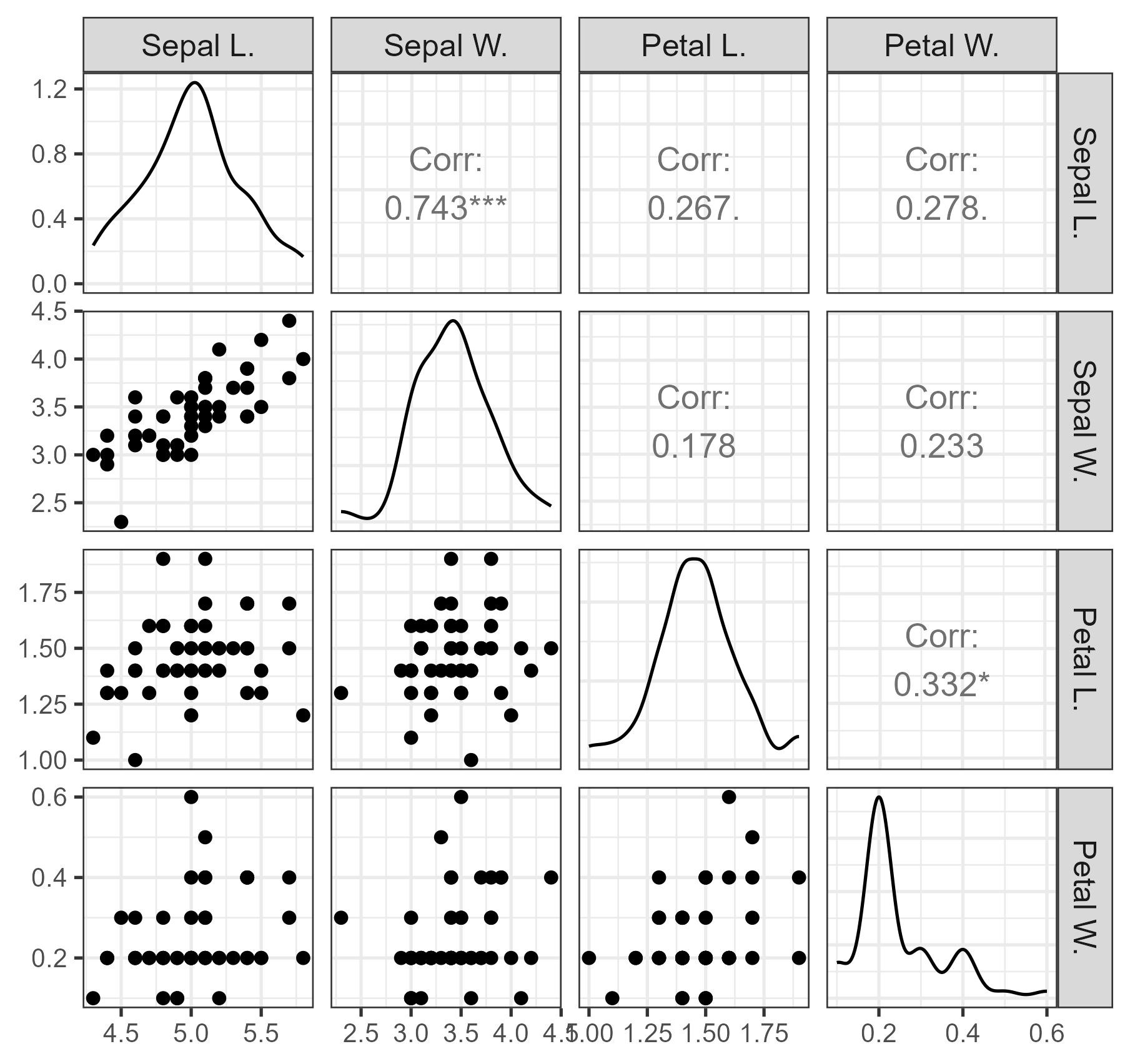
We specify the null cumulative distribution function, density, simulation routine, and parameter estimator:
pnull = function (x, p) {
    f = function(x)
       mvtnorm::pmvnorm(rep(-Inf, length(x)), x,
              mean = p[1:4],
              sigma = matrix(p[5:20], nrow = 4))
    if (!is.matrix(x)) return(f(x))
    apply(x, 1, f)
}
dnull = function (x, p) {
    f = function(x)
       mvtnorm::dmvnorm(x,
              mean = p[1:4],
              sigma = matrix(p[5:20], nrow = 4))
    if (!is.matrix(x)) return(f(x))
    apply(x, 1, f)
}
rnull = function(p) mvtnorm::rmvnorm(50,
              mean = p[1:4],
              sigma = matrix(p[5:20], nrow = 4))
phat = function(x) c(apply(x, 2, mean), cov(x))
The tests can then be run as follows, using a fixed random seed:
MDgof::gof_test(setosa, pnull, rnull, B = 1000,
        dnull = dnull, phat = phat, seed = 1234,
        doMethods = "all", maxProcessor = 1)
MDgof multivariate goodness-of-fit tests
Data: continuous | n = 50 | dimension = 4 | B = 1000
method statistic p.value
qKS 0.268 0.000
qK 0.278 0.000
qCvM 0.748 0.000
qAD 8.419 0.083
BR 1.309 0.564The individual tests give different results, which motivates illustrating the adjusted -value procedure. We use the same five methods in the adjusted test by specifying doMethods = "all":
MDgof::gof_test_adjusted_pvalue(setosa, pnull, rnull,
        B = 1000, dnull = dnull, phat = phat,
        seed = 1234, doMethods = "all", maxProcessor = 1)
p values of individual tests:
qKS : 0
qK : 0
qCvM : 0
qAD : 0.083
BR : 0.875
adjusted p value of combined tests: 0
qKS qK qCvM qAD BR Min p
0.000 0.000 0.000 0.083 0.875 0.000The adjusted -value is reported as zero at the simulation resolution used here; this is a Monte Carlo estimate, not an assertion that the probability is exactly zero. The example illustrates both the different responses of individual test statistics and the use of the adjusted -value routine. A substantive assessment of multivariate normality in these measurements is not the purpose of this example.
9.2 Goals in the English Premier League
For an illustration with discrete bivariate data, we compare the joint frequencies of goals scored by home and away teams in the English Premier League in 2020–21 and in the available portion of 2025–26. The original match results were obtained from Football-Data.co.uk (Football-Data.co.uk, 2026). The latter season was incomplete when the data were collected, so the comparison is intended only as a demonstration of the software, not as an assessment of changes in football tactics or scoring patterns.
For simplicity, the example uses the categories 0 through 4 goals for each team. Matches in which either team scored five or more goals are excluded, so the analysis applies only to the retained matches. To make the results independent of future changes to the source website, the 25-row frequency table is included directly in the replication material. It has columns vals_x and vals_y for home and away goals, and x and y for the corresponding frequencies in the two seasons.
goals_premier_league <- cbind(
  vals_x = rep(0:4, times = 5),
  vals_y = rep(0:4, each = 5),
  x = c(30,33,26,14,6, 38,40,27,13,4,
        23,33,7,7,3, 14,18,7,6,2, 3,4,3,2,0),
  y = c(27,22,29,27,2, 31,47,37,20,6,
        15,27,26,11,3, 10,9,10,3,2, 2,4,1,2,1)
)
We apply the eight tests available by default for these discrete data:
MD2sample::twosample_test(goals_premier_league,
                          B = 1000, seed = 1234)
MD2sample two-sample tests
Data: discrete | n.x = 363 | n.y = 374 | dimension = 2 | B = 1000
method statistic p.value
KS 0.1314 0.0040
K 0.1827 0.0020
CvM 0.4884 0.0410
AD 2.3511 0.0530
NN 3.0350 0.0400
AZ 0.2111 0.0040
BF 0.3149 0.0040
ChiSquare 33.1600 0.0445To illustrate simultaneous inference using the complete collection of eight discrete-data methods, we specify doMethods = "all" in twosample_test_adjusted_pvalue. Without this option, the routine uses four methods by default: Chi-square, Kolmogorov–Smirnov, Aslan–Zech, and Cramér–von Mises.
MD2sample::twosample_test_adjusted_pvalue(
    goals_premier_league, B = 1000, seed = 1234,
    doMethods = "all")
p values of individual tests:
KS: 0.004
K: 0.002
CvM: 0.041
AD: 0.053
NN: 0.04
AZ: 0.004
BF: 0.004
ChiSquare: 0.0445
adjusted p value of combined tests: 0.013The adjusted -value for these eight tests is 0.013. The example demonstrates the use of the discrete two-sample procedures and their combined calibration. Because the seasons have different coverage and the frequency table excludes high-scoring matches, no substantive conclusion about changes in Premier League goal-scoring patterns is drawn.
10 Discussion
Because the relative power of the procedures depends on the null distribution, the alternative, the dimension, and the sample size, the benchmark results should not be interpreted as general rankings. The simulation facilities provided by the packages allow users to compare procedures under scenarios relevant to their applications.
Multivariate goodness-of-fit and two-sample testing present a computational comparison problem as much as an implementation problem. The large number of available procedures reflects the fact that sensitivity to departures from the null varies with the geometry of the alternative, dimension, sample size, and treatment of nuisance parameters. Consequently, providing another isolated implementation of a test does not by itself solve the practical problem faced by analysts or the evaluation problem faced by researchers developing new methodology.
The contribution of MDgof and MD2sample is a common computational environment in which heterogeneous procedures can be applied, calibrated, compared, and benchmarked. Built-in statistics cover several methodological families and both continuous and discrete data. More importantly, user-defined statistics can enter the same testing, Monte Carlo power, simultaneous-inference, and benchmarking workflows. The deliberately parallel interfaces of the two packages make the computational structure of goodness-of-fit and two-sample studies similar from the user’s perspective even though their null-generation mechanisms differ.
The benchmark collections are not intended to identify a universally best test. Rather, they provide reproducible scenarios in which the strengths and weaknesses of competing statistics can be studied under common conditions. This is especially useful when a new statistic is proposed: the researcher can compare it with established procedures without writing a separate simulation infrastructure for every competitor.
There are also limitations. Some multivariate empirical-distribution-function statistics require computational approximations, and the cost of resampling-based calibration can be substantial for large samples or extensive benchmark grids. The framework therefore uses compiled code and parallel processing where appropriate, but computational burden remains method dependent. Future development can extend the collection of benchmark alternatives, incorporate additional testing families, and improve computational strategies for large or high-dimensional data.
In this sense, MDgof and MD2sample provide infrastructure for reproducible methodological comparison. They provide a common environment in which established and newly proposed multivariate goodness-of-fit and two-sample procedures can be implemented, evaluated, and compared under controlled simulation conditions.
Statements and Declarations
Funding. No funds, grants, or other support was received.
Competing interests. The author has no relevant financial or non-financial interests to disclose.
Generative AI use. OpenAI ChatGPT (GPT-5.6 Sol) was used during manuscript preparation for language and organizational assistance, consistency checking, and software coding and debugging assistance. All resulting text, code, numerical results, and references were reviewed and verified by the author, who takes full responsibility for the content of the manuscript.
Data and Code Availability
Data availability. The Fisher iris data are included with R. The English Premier League data used in Section 9.2 are publicly available from Football-Data.co.uk. The remaining numerical examples and simulation studies use data generated by the code and the MDgof and MD2sample packages described in the article.
Code availability. The MDgof and MD2sample packages are publicly available from CRAN. Code needed to reproduce the numerical examples is given in the article, and the benchmark-generating routines and case studies are included in the packages.
References
- Aldor-Noiman, S., Brown, L. D., Buja, A., Rolke, W., & Stine, R. A. (2013). The Power to See: A New Graphical Test of Normality. The American Statistician, 67(4), 249–260. https://doi.org/10.1080/00031305.2013.847865 ↩
- Anderson, T. W. (1962). On the Distribution of the Two-Sample Cramer-von Mises Criterion. The Annals of Mathematical Statistics, 33(3), 1148–1159. https://doi.org/10.1214/aoms/1177704477 ↩
- Anderson, T. W., & Darling, D. A. (1952). Asymptotic Theory of Certain “Goodness of Fit” Criteria Based on Stochastic Processes. The Annals of Mathematical Statistics, 23(2), 193–212. https://doi.org/10.1214/aoms/1177729437 ↩
- Aslan, B., & Zech, G. (2005). New test for the multivariate two-sample problem based on the concept of minimum energy. Journal of Statistical Computation and Simulation, 75(2), 109–119. https://doi.org/10.1080/00949650410001661440 ↩
- Bakshaev, A., & Rudzkis, R. (2015). Multivariate goodness-of-fit tests based on kernel density estimators. Nonlinear Analysis: Modelling and Control, 20(4), 585–602. https://doi.org/10.15388/na.2015.4.9 ↩
- Baringhaus, L., & Franz, C. (2004). On a new multivariate two-sample test. Journal of Multivariate Analysis, 88(1), 190–206. https://doi.org/10.1016/s0047-259x(03)00079-4 ↩
- Bickel, P. J., & Breiman, L. (1983). Sums of Functions of Nearest Neighbor Distances, Moment Bounds, Limit Theorems and a Goodness of Fit Test. The Annals of Probability, 11(1), 185–214. https://doi.org/10.1214/aop/1176993668 ↩
- Biswas, M., & Ghosh, A. K. (2014). A nonparametric two-sample test applicable to high dimensional data. Journal of Multivariate Analysis, 123, 160–171. https://doi.org/10.1016/j.jmva.2013.09.004 ↩
- Chen, H., & Friedman, J. H. (2017). A New Graph-Based Two-Sample Test for Multivariate and Object Data. Journal of the American Statistical Association, 112(517), 397–409. https://doi.org/10.1080/01621459.2016.1147356 ↩
- Cramér, H. (1928). On the composition of elementary errors: First paper: Mathematical deductions. Scandinavian Actuarial Journal, 1928(1), 13–74. https://doi.org/10.1080/03461238.1928.10416862 ↩
- Eddelbuettel, D., François, R., Allaire, J., Ushey, K., Kou, Q., Russell, N., Ucar, I., Bates, D., & Chambers, J. (2024). Rcpp: Seamless r and c++ integration [R package version 1.1.1-1.1]. https://CRAN.R-project.org/package=Rcpp ↩
- Fasano, G., & Franceschini, A. (1987). A multidimensional version of the Kolmogorov–Smirnov test. Monthly Notices of the Royal Astronomical Society, 225(1), 155–170. https://doi.org/10.1093/mnras/225.1.155 ↩
- Fisher, R. A. (1936). The use of multiple measurements in taxonomic problems. Annals of Eugenics, 7(2), 179–188. https://doi.org/10.1111/j.1469-1809.1936.tb02137.x ↩
- Football-Data.co.uk. (2026). Historical football match results data archive. ↩
- Franz, C. (2024). Cramer: Multivariate nonparametric cramer-test for the two-sample-problem [R package version 0.9-4]. https://CRAN.R-project.org/package=cramer ↩
- Friedman, J. H., & Rafsky, L. C. (1979). Multivariate Generalizations of the Wald-Wolfowitz and Smirnov Two-Sample Tests. The Annals of Statistics, 7(4), 697–717. https://doi.org/10.1214/aos/1176344722 ↩
- Gretton, A., Sejdinovic, D., Strathmann, H., Balakrishnan, S., Pontil, M., Fukumizu, K., & Sriperumbudur, B. K. (2012). Optimal kernel choice for large scale two sample tests. Advances in Neural Information Processing Systems (NIPS), 1205–1213. ↩
- Karatzoglou, A., Smola, A., Hornik, K., & Zeileis, A. (2004). kernlab - An S4 Package for Kernel Methods in R. Journal of Statistical Software, 11(9). https://doi.org/10.18637/jss.v011.i09 ↩
- Kolmogorov, A. N. (1933). Sulla determinazione empirica di una legge di distribuzione. Giornale Dell’Instituto Italiano Degli Attuari, 4, 83–91. ↩
- Kuiper, N. H. (1960). Tests concerning random points on a circle. Indagationes Mathematicae (Proceedings), 63, 38–47. https://doi.org/10.1016/s1385-7258(60)50006-0 ↩
- von Mises, R. (1928). Wahrscheinlichkeit Statistik und Wahrheit. Springer Berlin Heidelberg. https://doi.org/10.1007/978-3-662-36230-3 ↩
- Pan, W., Tian, Y., Wang, X., & Zhang, H. (2018). Ball Divergence: Nonparametric two sample test. The Annals of Statistics, 46(3), 1109–1137. https://doi.org/10.1214/17-aos1579 ↩
- Pettitt, A. N. (1976). A two-sample anderson-darling rank statistic. Biometrika, 63(1), 161–168. ↩
- Puritz, C., Ness-Cohn, E., & Braun, R. (2023). fasano.franceschini.test: An Implementation of a Multivariate KS Test in R. The R Journal, 15(3), 159–171. https://doi.org/10.32614/rj-2023-067 ↩
- Rayner, J. C. W., Thas, O., & Best, D. J. (2009). Smooth tests of goodness of fit. Wiley. ↩
- Ripley, B. D. (1976). The second-order analysis of stationary point processes. Journal of Applied Probability, 13(2), 255–266. https://doi.org/10.2307/3212829 ↩
- Rizzo, M. L., & Székely, G. J. (2024). Energy: E-statistics: Multivariate inference via the energy of data [R package version 1.7-12]. https://CRAN.R-project.org/package=energy ↩
- Rolke, W. (2025). Rgof and R2sample: Testing and Benchmarking for the Univariate Goodness-of-Fit and Two-Sample Problems. The R Journal, 17(3), 138–161. https://doi.org/10.32614/rj-2025-027 ↩ 1 2
- Rolke, W. (2026a). MD2sample: Various methods for the two-sample problem in D > 1 dimensions [R package version 1.4.2]. https://doi.org/10.32614/CRAN.package.MD2sample
- Rolke, W. (2026b). MDgof: Various methods for the goodness-of-fit problem in D > 1 dimensions [R package version 1.2.1]. https://doi.org/10.32614/CRAN.package.MDgof
- Smirnov, N. V. (1939). Estimate of deviation between empirical distribution functions in two independent samples. Bulletin of Moscow University, 2, 3–16. ↩
- Thas, O. (2010). Comparing distributions. Springer. ↩
- Westfall, P. H., & Young, S. S. (1993). Resampling-based multiple testing: Examples and methods for p-value adjustment. John Wiley & Sons. ↩
Cite this article
Rolke, W. (2026). A Computational Framework for Multivariate Goodness-of-Fit and Two-Sample Testing: MDgof and MD2sample. Journal of Reproducible Statistics, 1, 8. https://doi.org/10.68365/jrepstat.2026.8
Rolke, Wolfgang. 2026. “A Computational Framework for Multivariate Goodness-of-Fit and Two-Sample Testing: MDgof and MD2sample.” Journal of Reproducible Statistics 1: 8. https://doi.org/10.68365/jrepstat.2026.8.
Rolke W. A Computational Framework for Multivariate Goodness-of-Fit and Two-Sample Testing: MDgof and MD2sample. Journal of Reproducible Statistics. 2026;1:8. doi:10.68365/jrepstat.2026.8
Rolke, W. (2026) “A Computational Framework for Multivariate Goodness-of-Fit and Two-Sample Testing: MDgof and MD2sample,” Journal of Reproducible Statistics, 1, p. 8. Available at: https://doi.org/10.68365/jrepstat.2026.8.
doi: https://doi.org/10.68365/jrepstat.2026.8
Downloads
https://doi.org/10.68365/jrepstat.2026.8 also supports content negotiation, so reference managers can fetch the citation from the DOI directly. The exports above work without it.