1 Introduction

A multivariate full conformal prediction (FullCP) procedure accepts or rejects each candidate response $t$ through an exact conformal comparison, and the collection of accepted candidates is the prediction region studied here. Under the standard exchangeability framework, with i.i.d. sampling as a canonical special case, conformal prediction supplies its usual finite-sample marginal validity (Shafer & Vovk, 2008; Vovk et al., 2005). This paper addresses a different layer of the problem: the geometry of that exact accepted set and how to represent it faithfully. The validity guarantee is inherited background; the contribution is score-specific exact-set geometry and deterministic reconstruction error control.

The present analysis uses the response-only special case of exchangeable conformal prediction: the observed examples are $Y_1,\ldots,Y_m$, with no covariates and no fitted predictive model. This restriction isolates the exact-set geometry induced by the score itself from the additional candidate dependence introduced by predictive-model fitting. Shafer & Vovk (2008) discuss the corresponding special case in which prediction is based on past examples without informative features of the new object. By contrast, several recent multivariate conformal methods formulate prediction for regression pairs $(X,Y)$ and/or incorporate fitted or pre-trained predictors (Diquigiovanni et al., 2022; Gan & Liu, 2025; Johnstone & Ndiaye, 2025). In refitted regression-based FullCP, the trial response can also enter the fitted predictor through the augmented training data (Lei et al., 2018), so the resulting score comparisons can depend on the trial value through model fitting as well as through direct score evaluation. Accordingly, Theorem 1 gives an exact characterization of the response-only score-induced setting studied here; it does not establish common-center geometry for refitted regression-based FullCP.

For example, at a fixed forecast context one may have exchangeable historical low-dimensional multivariate outcomes, with no predictor refit as the trial response varies. The empirical energy-score FullCP region can then be used directly for reporting or downstream candidate-level decisions.

That distinction matters in more than one response dimension. An exact FullCP region can be nonconvex, while a finite collection of directional boundary searches leaves uncertainty between sampled directions. Replacing the resulting boundary by an ellipse or convex hull may be convenient, but if the exact region is nonconvex then convexification can enlarge it and add candidates rejected by the exact conformal comparison. Such an enlargement is not claimed here to destroy marginal coverage validity; rather, it is no longer a faithful representation of the exact accepted set and can change its size, shape, and candidate-level decisions.

For the empirical energy-form pairwise score considered below, the leave-one-out algebra supplies a stronger structure than candidate-score convexity. Each training-versus-candidate comparison becomes exactly a pairwise-dissimilarity sublevel condition. Under the stated diagonal and attainment assumptions, all comparison regions contain a common Fréchet-type minimizer; when those comparison regions are convex, the nontrivial exact FullCP vote aggregate is star-shaped about that same point. Star-shapedness is the useful middle ground: the aggregate need not be convex, but every ray from the common center has a single radial exit, so the whole region can be represented ray by ray.

Power distances $\rho_\beta(x,y)=\lVert x-y\rVert ^\beta$ provide the main concrete family. Their deterministic common-center geometry holds for $\beta\ge1$. In one dimension at $\beta=1$, the score has the usual energy representation of the continuous ranked probability score (CRPS) (Gneiting & Raftery, 2007); for the fixed-bin empirical construction studied by Toccaceli (2026, ​Sections 8.1 and 8.3), the score geometry proves that every nontrivial exact FullCP set is a nonempty closed interval. This CRPS result is a recognizable specialization of the multivariate mechanism, not a new scoring-rule theorem.

The radial representation becomes certifiable on the regular range $1<\beta<2$. Along each direction, the exact FullCP radius is an order statistic of the component comparison-set radii. Explicit score-derived Lipschitz bounds on those radii then turn finitely many certified ray searches into global lower and upper radial envelopes. The envelope width combines the one-dimensional search tolerance with a directional covering term, and the same-center radial sandwich yields deterministic Hausdorff error bounds. Thus finite-direction reconstruction is accompanied by a global approximation certificate rather than only a plotted collection of rays.

The paper makes three contributions. First, it gives the exact score-difference reduction, common-center comparison geometry, and star-shaped aggregation, including the exact univariate empirical-CRPS interval result. Second, it identifies the radial order-statistic interface and, for $1<\beta<2$, explicit data-checkable radial regularity that makes finite-direction certification possible. Third, it derives a focuswise radial certificate that is deterministically no looser than a generic center-based benchmark and assesses the resulting certificate tightness and nonconvexity diagnostics in a frozen staged two-dimensional study. The analytic example in Section 4 shows explicitly why preserving nonconvexity can matter before the certification machinery is introduced.

The scope is deliberately limited. The geometric statements are specific to the score structure and assumptions developed here; no generic theorem for arbitrary FullCP regions is claimed. The paper does not add a conformal coverage theorem, and response-dependent adaptive partition questions remain outside scope. Directional covering restricts practical certification to low-dimensional multivariate outputs, and no runtime superiority is asserted. The numerical study is descriptive for its frozen designs rather than an estimate of how often nonconvexity occurs in a population of FullCP problems.

The standard variogram score used in multivariate forecast evaluation is not of the empirical observation-pair energy-form V-statistic form assumed in Theorem 1, so Theorem 1 does not directly cover it. This scope statement does not rule out analogous geometry for other variogram constructions.

Root finding and bisection for conformal sets predate this work (Ndiaye & Takeuchi, 2023), as does multi-output reconstruction from finitely many search directions (Johnstone & Ndiaye, 2025). In the latter framework, star-shapedness can be imposed as a structural condition and sampled boundary points can be fit by convex objects; here the common star center is instead derived from the score before directional approximation. Classical radius-$R$ supporting-ball geometry (Balashov & Golubev, 2012) and McShane–Whitney Lipschitz-extension formulas (Arnau et al., 2023) are used later as inherited tools after the score-specific bounds are established. Other certified FullCP approximations use different error metrics and scopes (Razafindrakoto et al., 2026b, 2026a). A companion Lean 4 development checks selected discrete and algebraic components of the present results; the multivariate regularity, adaptive-partition, and coverage questions are outside that formalization.

Section 2 develops the exact score-induced FullCP geometry. Section 3 specializes to power distances, isolates the empirical-CRPS interval result, and gives the exact radial order-statistic representation. Section 4 gives the analytic nonconvex witness before Section 5 develops certified reconstruction for $1<\beta<2$. Section 6 reports the staged numerical assessment, Section 7 records computational and endpoint limitations, and Section 8 synthesizes the scope. Appendices A–D contain the $\beta=1$ segment pathology, a three-point robustness witness, the detailed technical regularity calculations, and numerical protocol and reproducibility details.

2 Exact Score-Induced Full-Conformal Geometry

The setup can be read as a voting rule. For each candidate $t$, training observation $j$ contributes one comparison vote when its leave-one-out score is at least the candidate score; the exact FullCP region consists of candidates receiving enough such votes. The notation below makes that rule explicit before exploiting the score algebra.

Let $m\ge1$, $d\ge1$, and let $y_1,\ldots,y_m\in\mathbb R^d$. For a function $$\rho:\mathbb R^d\times\mathbb R^d\to\mathbb R$$ and an empirical distribution $$\widehat F=\frac1m\sum_{r=1}^m\delta_{z_r},$$ define the energy-form pairwise score $$S_\rho(\widehat F,y) = \frac1m\sum_{r=1}^m\rho(z_r,y) - \frac1{2m^2}\sum_{r,s=1}^m\rho(z_r,z_s).$$ The second term uses the empirical V-statistic normalization $1/(2m^2)$; no off-diagonal normalization is used.

For a candidate $t\in\mathbb R^d$, augment the observed responses by $$x_i(t)=y_i,\qquad i=1,\ldots,m, \qquad x_{m+1}(t)=t.$$ For $r=1,\ldots,m+1$, let $$\widehat F_{-r,t} = \frac1m \sum_{\substack{s=1\\s\ne r}}^{m+1} \delta_{x_s(t)}, \qquad \alpha_r(t) = S_\rho\!\left(\widehat F_{-r,t},x_r(t)\right),$$ and write $$\alpha(t)=\alpha_{m+1}(t).$$ For $j=1,\ldots,m$, define the comparison region $$I_j=\{t:\alpha_j(t)\ge\alpha(t)\}.$$ Thus score ties are accepted as comparison votes. Let $$N(t)=\sum_{j=1}^m\mathbf 1\{t\in I_j\}, \qquad p(t)=\frac{1+N(t)}{m+1},$$ and use throughout the strict conformal convention $$\Gamma^\varepsilon=\{t:p(t)>\varepsilon\}.$$ For $0\le\varepsilon<1$, set $$k=\lfloor(m+1)\varepsilon\rfloor.$$ Thus the exact endpoint regimes are $$k=0 \quad\left(0\le\varepsilon<\frac1{m+1}\right) \Longrightarrow \Gamma^\varepsilon=\mathbb R^d,$$ while $1\le k\le m$ is the nontrivial vote-threshold regime; in that regime the integer-valued vote count gives the exact equivalence $$\Gamma^\varepsilon=\{t:N(t)\ge k\}.$$ At $\varepsilon=1$, the strict convention gives $\Gamma^1=\varnothing$. These endpoint, tie, and threshold conventions will not be repeated inside later formal statements.

Candidate-score convexity is not sufficient. To see why the score-specific structure below is needed, temporarily replace the energy-form score by the generic reference-sample-symmetric nonconformity rule $$A(z;Z) = \frac1{|Z|} \sum_{w\in Z}|z-w^2| = \frac1{|Z|} \sum_{w\in Z}\ell(z,w), \qquad \ell(u,v)=|u-v^2|.$$ The rule is symmetric in the reference multiset $Z$, and $\ell(\,\cdot\,,v)$ is convex for every fixed $v$.

Take $m=2$ and $y_1=y_2=2$. For a candidate $t$, its score is $$\widetilde\alpha(t) = A(t;\{2,2\}) = |t-4|,$$ which is convex, whereas the two training scores coincide: $$\widetilde\alpha_1(t) = \widetilde\alpha_2(t) = A(2;\{2,t\}) = 1+\frac12|2-t^2|.$$ A direct piecewise calculation gives $$\widetilde\alpha_j(t)\ge\widetilde\alpha(t) \quad\Longleftrightarrow\quad t\le-4 \quad\text{or}\quad t\ge2.$$ Thus the corresponding full-conformal $p$-value is $$\widetilde p(t) = \begin{cases} 1, & t\in(-\infty,-4]\cup[2,\infty),\\[1mm] 1/3, & -4<t<2. \end{cases}$$ At $\varepsilon=1/2$, using the strict convention $\widetilde p(t)>\varepsilon$, $$\widetilde\Gamma^{1/2} = (-\infty,-4]\cup[2,\infty),$$ which is disconnected. Equality holds at $t=-4$ and $t=2$, so both endpoints are included because comparison votes use $\ge$.

This example is not asserted to arise from a proper distributional scoring rule. Its role is narrower: candidate-score convexity is not sufficient for connected FullCP regions, even within the empirical-average form with a loss convex in its candidate argument.

The following result isolates the stronger algebraic and geometric structure that is sufficient for the energy-form score.

Before stating the result, define $$d_j=\sum_{i\ne j}\rho(y_j,y_i), \qquad F(t)=\sum_{i=1}^m\rho(t,y_i).$$

The theorem separates three logically distinct ingredients. Symmetry and a constant diagonal suffice for the exact comparison identity. The diagonal lower bound and attainment of $F$ give a common point of all comparison regions. Convexity of the individual comparison regions is needed only for the final segment argument. The preceding counterexample shows that convexity of the candidate score itself is not a substitute for this comparison-set structure. The resulting $k$-coverage set can be star-shaped without being convex; Section 4 gives an explicit analytic example.

3 Power Distances, Empirical CRPS, and Radial Representation

Consider the power-distance dissimilarity $$\rho_\beta(x,y)=\lVert x-y\rVert ^\beta.$$ This family gives a concrete deterministic geometry and, on a narrower parameter range, the conventional energy-score interpretation.

Finite exits and the $m=1$ degeneracy. When $m=1$, $G_1$ is the empty sum and $d_1=0$, so $I_1=\mathbb R^d$ and finite-radius reconstruction is degenerate. When $m\ge2$, each $G_j$ contains at least one coercive term and $I_j=\{G_j\le d_j\}$ is bounded, so every ray from a common center has a finite exit.

For $d=1$ and $\beta=1$, this score is exactly the fixed-bin empirical CRPS score used by Toccaceli (2026, Section 8.1). The univariate case deserves a separate formal statement because it gives the exact interval property for that construction. Write the ordered observations as $$y_{(1)}\le\cdots\le y_{(m)}$$ and define the full empirical median set $$\mathcal M = \arg\min_t F_1(t) = \left[ y_{(\lceil m/2\rceil)}, y_{(\lfloor m/2\rfloor+1)} \right].$$

For clarity, the augmented fixed-bin construction sets $$x_i(t)=y_i\quad(i\le m),\qquad x_{m+1}(t)=t, \qquad \widehat F_{-r,t}=\frac1m\sum_{\substack{s=1\\s\ne r}}^{m+1}\delta_{x_s(t)}.$$ Its score is $$\operatorname{CRPS}(\widehat F_{-r,t},x_r(t)) =\frac1m\sum_{\substack{s=1\\s\ne r}}^{m+1}|x_s(t)-x_r(t)| -\frac1{2m^2}\sum_{\substack{s,\ell=1\\s,\ell\ne r}}^{m+1}|x_s(t)-x_\ell(t)|.$$ This is exactly the energy-form score with $\rho(x,y)=|x-y|$ and the same empirical V-statistic normalization.

This proves the single-interval property reported for Toccaceli’s fixed-bin empirical-CRPS construction. The interval conclusion follows from the deterministic comparison geometry and does not by itself extend to proper distributional scoring rules in general.

Scoring-rule range. Under the conventional distributional energy-score interpretation, with $$\mathcal P_\beta = \left\{P:\int\lVert x\rVert ^\beta\,dP(x)<\infty\right\},$$ the power-distance energy score is strictly proper on the appropriate finite-moment class for $0<\beta<2$ (Gneiting & Raftery, 2007). At $\beta=2$ it is proper but not strictly proper and its expected score depends only on the forecast mean; for $\beta>2$ the Euclidean distance-power energy-form score is not proper. Thus strict propriety overlaps the deterministic star-shaped geometry on $1\le\beta<2$. These are classical scoring-rule facts and do not enlarge the deterministic claims above.

Lower-boundary sharpness. The deterministic conclusion should not be extended below $\beta=1$. With $$m=3, \qquad \beta=\frac12, \qquad (y_1,y_2,y_3)=(-1,0,2),$$ the unique Fréchet minimizer is $c=0$, yet at $\varepsilon=0.8$ the exact prediction set contains $0$ and $1$ while rejecting $0.5$. Thus it is not star-shaped about $c$.

For the remainder of the radial development, assume the comparison sets are star-shaped about a common center $c$ and define, for $u\in\mathbb S^{d-1}$, $$R_j(u)=\sup\{r\ge0:c+ru\in I_j\}.$$ For a nontrivial threshold, define likewise $$R_\varepsilon(u)=\sup\{r\ge0:c+ru\in\Gamma^\varepsilon\},$$ and let $R_{(1)}(u)\le\cdots\le R_{(m)}(u)$ be the ascending order statistics of the component exits.

The endpoint conventions remain those fixed in Section 2: $k=0$ gives $\Gamma^\varepsilon=\mathbb R^d$ and hence $R_\varepsilon\equiv+\infty$, while $\varepsilon=1$ gives the empty set. For power distances with $m=1$, $I_1=\mathbb R^d$ and $R_1\equiv+\infty$, so finite radial reconstruction begins at $m\ge2$. At $\beta=1$, exact common-center star-shaped geometry remains valid but unconditional global radial Lipschitzness can fail; Appendix A gives an exact discontinuous example.

4 Why Preserving Nonconvexity Can Matter

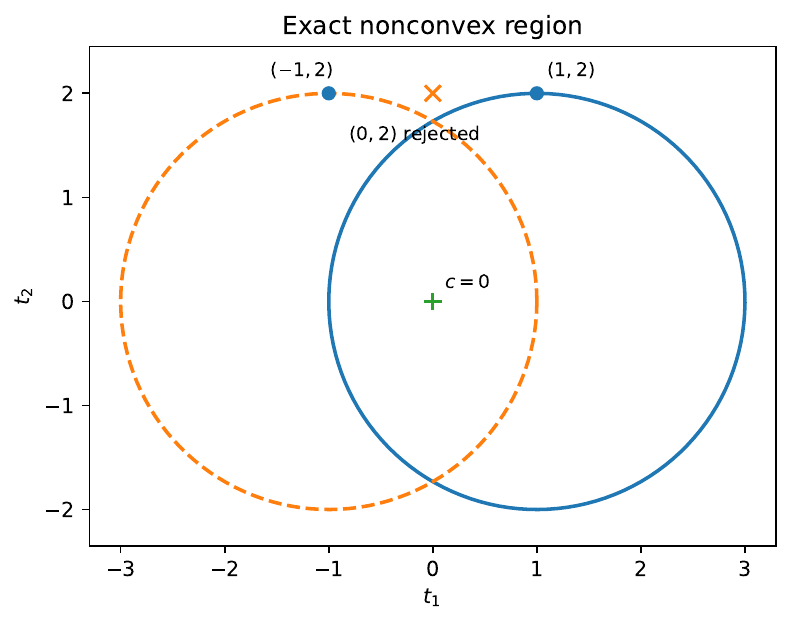
For this section, write $\Gamma=\Gamma^\varepsilon$. A two-dimensional analytic example makes the distinction between star-shapedness and convexity explicit before the reconstruction machinery is introduced. Let $$d=2, \qquad m=2, \qquad \beta=\frac32,$$ with $$y_1=(-1,0), \qquad y_2=(1,0), \qquad \varepsilon=\frac12.$$ Then $k=\lfloor3/2\rfloor=1$. For $j=1$, the comparison objective contains only the distance to $y_2$, and $d_1=\lVert y_1-y_2\rVert ^{3/2}=2^{3/2}$. Therefore $$I_1=B(y_2,2), \qquad I_2=B(y_1,2),$$ and the one-vote prediction region is exactly $$\Gamma^\varepsilon=I_1\cup I_2.$$ The origin is a common center. With $$u(\theta)=(\cos\theta,\sin\theta),$$ the two ball exits are $$\cos\theta+\sqrt{\cos^2\theta+3} \quad\text{and}\quad -\cos\theta+\sqrt{\cos^2\theta+3},$$ so the union has exact radial function $$R(\theta) = |\cos\theta|+\sqrt{\cos^2\theta+3}.$$ This set is star-shaped about $0$ but nonconvex: $$(-1,2),(1,2)\in\Gamma^\varepsilon, \qquad (0,2)\notin\Gamma^\varepsilon.$$

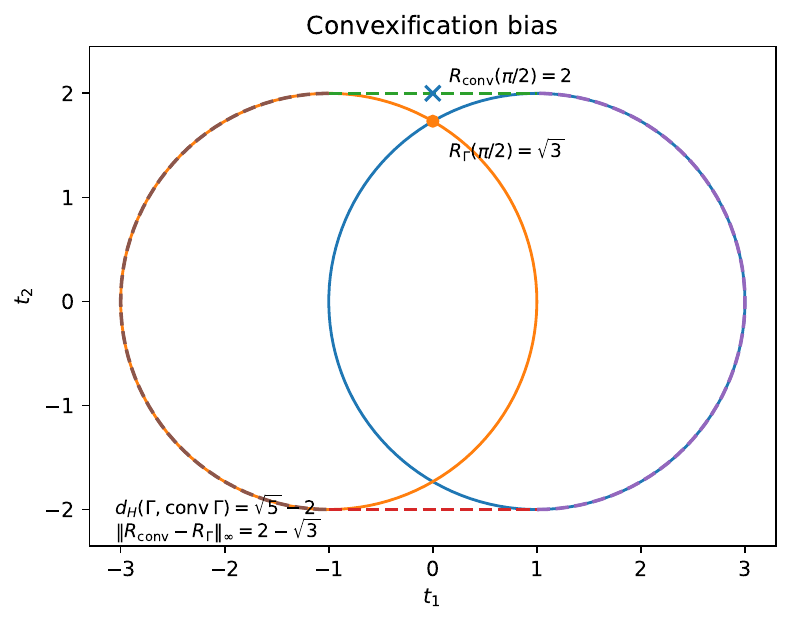
Its convex hull is the stadium $$\operatorname{conv}\Gamma^\varepsilon = [-e_1,e_1]+B(0,2).$$ Direct geometry gives the exact radial convexification discrepancy $$\lVert R_{\operatorname{conv}\Gamma}-R_\Gamma\rVert _\infty =2-\sqrt3,$$ and the exact Hausdorff discrepancy $$d_H(\Gamma,\operatorname{conv}\Gamma) =\sqrt5-2.$$ The latter is attained at the midpoint of the top or bottom flat portion of the stadium boundary, whose distance to either radius-$2$ component ball is $\sqrt5-2$. These positive discrepancies are properties of this analytic witness; they do not imply that convex reconstruction is inappropriate in every conformal problem. In particular, because the convex hull is a superset of the exact accepted set, no claim is made that this enlargement itself destroys marginal coverage validity. The point is fidelity: convexification adds candidates rejected by the exact comparison and therefore changes the exact FullCP region.

For a same-scale comparison, the analytic union has area and equivalent-area radius $$A_\Gamma=\frac{16\pi}{3}+2\sqrt3, \qquad r_{\textrm{eq}}=\sqrt{\frac{16}{3}+\frac{2\sqrt3}{\pi}} \approx2.5369255259.$$ Thus its radial gap $2-\sqrt3$ has normalized magnitude $$\frac{2-\sqrt3}{r_{\textrm{eq}}}\approx0.1056196525.$$ This analytic example is a stress-test and existence illustration: convexification can be materially nonfaithful, but it makes no representative-magnitude claim. In contrast, conditional on ROBUST_WITNESS, the frozen numerical study in Section 6 had normalized radial-gap median $0.00137$, 90th percentile $0.00626$, and maximum $0.01770$. The frozen DGPs therefore had often-detectable but usually shallow nonconvexity. At these observed magnitudes convexification may be negligible for coarse visualization or coarse summaries, while exact boundary-near candidate membership can nevertheless change.

(A)

(B)

The nonconvexity is not an artifact of using only two observations. In the three-point example of Appendix B with $m=3$, $\beta=3/2$, and $k=2$, two symmetric endpoints are accepted while their midpoint is rejected, with nonzero comparison margins. The numerical margins are recorded only in the appendix. The computational implication is that the natural exact target is the star-shaped radial function, rather than a convex surrogate, which motivates the certified reconstruction developed next.

5 Certified Radial Reconstruction for $1<\beta<2$

We now restrict to $m\ge2$, $1<\beta<2$, and a nontrivial threshold $1\le k\le m$. The goal is to turn the exact radial representation into a global certificate from finitely many ray searches. Throughout, $$B(a,R)=\{x\in\mathbb R^d:\lVert x-a\rVert \le R\}$$ denotes the closed Euclidean ball.

5.3 Set certification and implementation

Define $$\underline\Gamma = \{c+ru:u\in\mathbb S^{d-1},\ 0\le r\le\underline R(u)\},$$ and $$\overline\Gamma = \{c+ru:u\in\mathbb S^{d-1},\ 0\le r\le\overline R(u)\}.$$

Corollary 3 (Certified inner and outer FullCP regions). The finite-direction envelopes satisfy $$\underline\Gamma\subseteq\Gamma^\varepsilon\subseteq\overline\Gamma.$$ Moreover, $$d_H(\underline\Gamma,\Gamma^\varepsilon) \le \lVert R_\varepsilon-\underline R\rVert _\infty \le \delta+2\widetilde Lh_{\mathcal U},$$ $$d_H(\Gamma^\varepsilon,\overline\Gamma) \le \lVert \overline R-R_\varepsilon\rVert _\infty \le \delta+2\widetilde Lh_{\mathcal U},$$ and $$d_H(\underline\Gamma,\overline\Gamma) \le \lVert \overline R-\underline R\rVert _\infty \le \delta+2\widetilde Lh_{\mathcal U}.$$

Proof. The radial sandwich gives the set inclusions directly. For two nested same-center radial sets, any point of the larger set can be moved along its own ray to the smaller radial boundary, so the directed distance is bounded by the radial-function gap in that direction. Taking suprema gives the three inequalities; Appendix C records the full derivation. ◻

Operationally, the directional intervals require no new per-ray search algorithm. For fixed $u$, membership along $c+ru$ is an initial interval for each comparison set, so $N(c+ru)$ is nonincreasing in $r$. The finite bound $H_{\max}=\max_jH_j$ brackets every component exit. If the vote threshold still holds at $H_{\max}$, the exact aggregate exit is $H_{\max}$; otherwise bisection between the accepted center and rejected outer radius produces a certified bracket of width at most $\delta$, using the root-search architecture of Ndiaye & Takeuchi (2023) and Johnstone & Ndiaye (2025). A numerically chosen center $\tilde c$ is sufficient whenever all inequalities $G_j(\tilde c)\le d_j$ are themselves certified; the search radii $H_j$ must then be recomputed, whereas $U_{ij}$ and the tightened regularity constants do not depend on the chosen common center; $L_{\textrm{old}}$ remains center-dependent if retained for comparison. No runtime improvement is claimed.

The same analytic example from Section 4 illustrates the certificate after the regularity result is available.

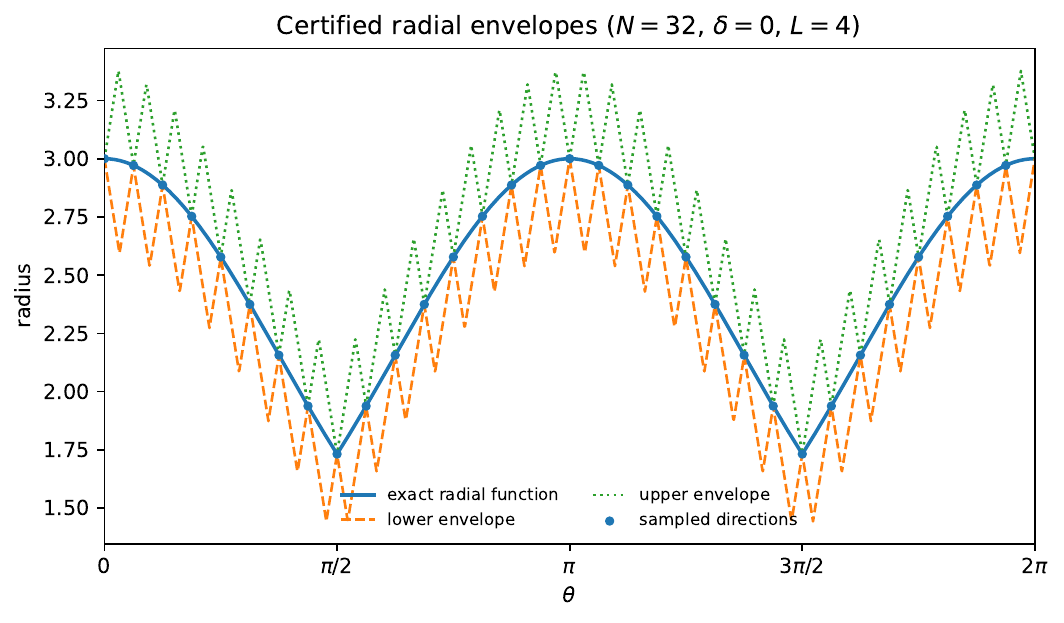
For this example, $U_{12}=U_{21}=2$, so $\widetilde M_j=(3/2)\sqrt2$, $\widetilde\lambda_j=3/(4\sqrt2)$, and $\widetilde L=2\widetilde M_j/\widetilde\lambda_j=8$. The radius-$2$ ball geometry itself gives the rigorous bound $L=4$ used in Figure 2. Finally, writing the exact radius as a function of $s=|u_1|\in[0,1]$ gives $$f(s)=s+\sqrt{s^2+3}, \qquad f'(s)=1+\frac{s}{\sqrt{s^2+3}}\le\frac32,$$ and $u\mapsto|u_1|$ is $1$-Lipschitz in chord distance, so $L_{\textrm{direct}}=3/2$. The sequence $$16\ \longrightarrow\ 8\ \longrightarrow\ 4\ \longrightarrow\ \frac32$$ uses successively more problem-specific information; in particular, the tightened general certificate gives $8$, not $4$ or $3/2$.

The reconstruction results stop at $1<\beta<2$. Comparison-set convexity itself holds for every $\beta\ge1$, but Appendix A shows that exact common-center geometry at $\beta=1$ does not imply unconditional global radial Lipschitzness.

6 Numerical Assessment

The numerical study assesses certificate tightness and the detectability and radial magnitude of nonconvexity under frozen two-dimensional designs; it is not a coverage experiment and its detection frequencies are not estimates of population prevalence. The study was staged. The initial smoke run used 5 independent clouds per $(m,\text{data-generating process (DGP)})$ cell, 40 total, and expansion to 20 independent clouds per cell was allowed only after the seven advance-declared engineering and numerical gates listed in Appendix D passed; soft flags did not automatically block expansion. After those gates passed, the expanded-production $\beta/q_{\textrm{vote}}$ grid, seed mapping, and no-post-hoc rule were frozen before any expanded-run results were observed. The original five clouds in each cell were retained in the final 20, so the final 160 clouds include the original 40 smoke clouds.

The 20 clouds per $(m,\mathrm{DGP})$ cell were the staged descriptive expansion size, not a target-precision sample size. For each $m\in\{10,25\}$, the final dataset contained 20 independent clouds from each of four designs—an isotropic Gaussian, a rotated anisotropic Gaussian, a symmetric Gaussian mixture, and a standardized bivariate $t_3$ distribution.¹ The fixed grid was $\beta\in\{1.1,1.5,1.9\}$ and $q_{\textrm{vote}}\in\{0.10,0.20,0.50\}$, with each cloud reused across the $\beta/q_{\textrm{vote}}$ settings. The threshold target determines $$k=\max\{1,\lfloor q_{\textrm{vote}}m+1/2\rfloor\},$$ whose corresponding strict-conformal $\varepsilon$ interval is $[k/(m+1),(k+1)/(m+1))$. Certificate summaries therefore operate at the 480 cloud–$\beta$ level, whereas witness and radial summaries use repeated $\beta/q_{\textrm{vote}}$ configurations within cloud; the resulting 1,440 cloud–$\beta$–$k$ rows are not independent observations. Values at 16,384 directions occur only for cases that triggered the prespecified fallback rule in Appendix D.

Across the 480 cloud–$\beta$ analyses, the median ratio $\widetilde L/L_{\textrm{old}}$ was $0.966$, with interquartile range (IQR) approximately $[0.941,0.976]$, equivalent to a median tightening of $3.39\%$. Descriptively, the median ratio was $0.941$ (IQR $[0.932,0.955]$) for $m=10$ and $0.975$ (IQR $[0.972,0.980]$) for $m=25$; no inferential significance is attached to this difference. Consistent with the deterministic ordering in Proposition 2, $\widetilde L\le L_{\textrm{old}}$ in every one of the 480 analyses. Figure 3 summarizes the certificate comparison.

To fix the numerical scale, on the full validation mesh define $$W_{\max}(L,N) = \max_u\left[\overline R_{L,N}(u)-\underline R_{L,N}(u)\right].$$ On the 8,192-direction radial mesh, with radial values $\widehat R_i$, define $$A_\Gamma=\frac{\pi}{8192}\sum_{i=1}^{8192}\widehat R_i^2, \qquad r_{\textrm{eq}}=\sqrt{A_\Gamma/\pi}.$$ For the operational target $W_{\max}\le0.10\,r_{\textrm{eq}}$, neither certificate achieved the target at $N\le128$ in the expanded study. At $N=256$, the descriptive fraction was $128/1440=8.89\%$ for $L_{\textrm{old}}$ and $165/1440=11.46\%$ for $\widetilde L$. These fractions aggregate repeated cloud–$\beta$–$k$ configurations and are not independent-observation estimates. The tilde envelope width was smaller in all 7,200 declared analysis-by-$N$ comparisons, as expected from the deterministic certificate ordering.

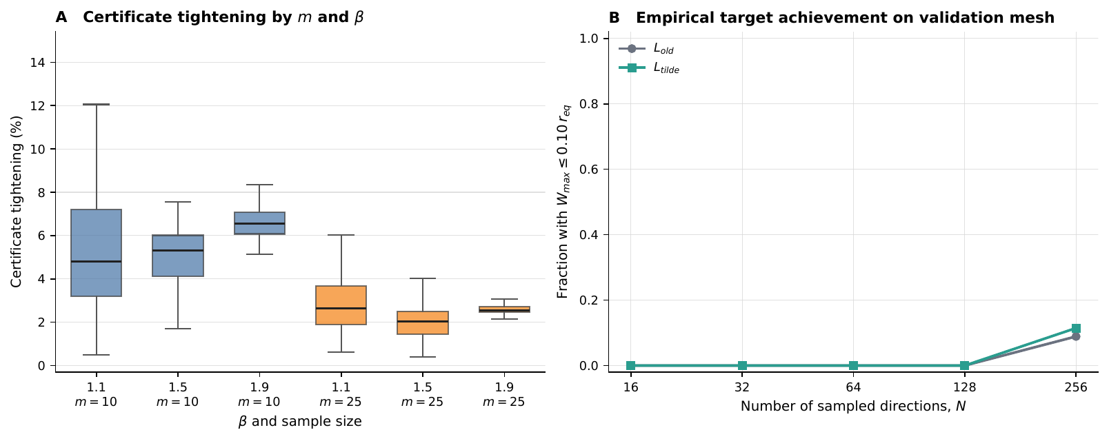
For the frozen 4,096-direction diagnostic mesh, the radial brackets are $\widehat R_i\pm e_i$, and we write the finite-grid lower proxy as $$L_{\textrm{sec}}^{-} = \max_{i\ne j} \frac{\max\{0,|\widehat R_i-\widehat R_j|-e_i-e_j\}} {\lVert u_i-u_j\rVert }.$$ This is a finite-grid lower proxy, not the true Lipschitz constant.² The median certificate-to-finite-grid-lower-proxy ratio was $108.8$ (IQR $[63.5,201.4]$) for $L_{\textrm{old}}$ and $105.9$ (IQR $[59.9,193.9]$) for $\widetilde L$. Substantial residual slack remains relative to the finite-grid lower proxy. The focuswise tightening therefore removes only part of the gap visible against this numerical lower diagnostic.

Figure 4 reports robust-witness detection rates over the prespecified grid. Operationally, the detector forms witness hulls from the common center and genuinely accepted radial lower endpoints, inspects hull edges joining nonadjacent angular samples, and searches convex combinations after any required inward endpoint backoff; ROBUST_WITNESS requires both endpoints to be robustly accepted and the convex-combination point to be robustly rejected under the stored aggregate-margin intervals, with a component/direct radial cross-check. SUGGESTIVE records a prescribed candidate that remains unresolved after the frozen refinement procedure, whereas NONE_DETECTED means only that this finite diagnostic found no witness; Appendix D gives the search details. Each fixed $\beta/q_{\textrm{vote}}$ cell contains exactly 160 independent clouds, and the cellwise detection rates range from $40.0\%$ to $81.2\%$. At the independent-cloud level, $155/160$ clouds yielded at least one robust witness somewhere among the nine prespecified $\beta/q_{\textrm{vote}}$ configurations. 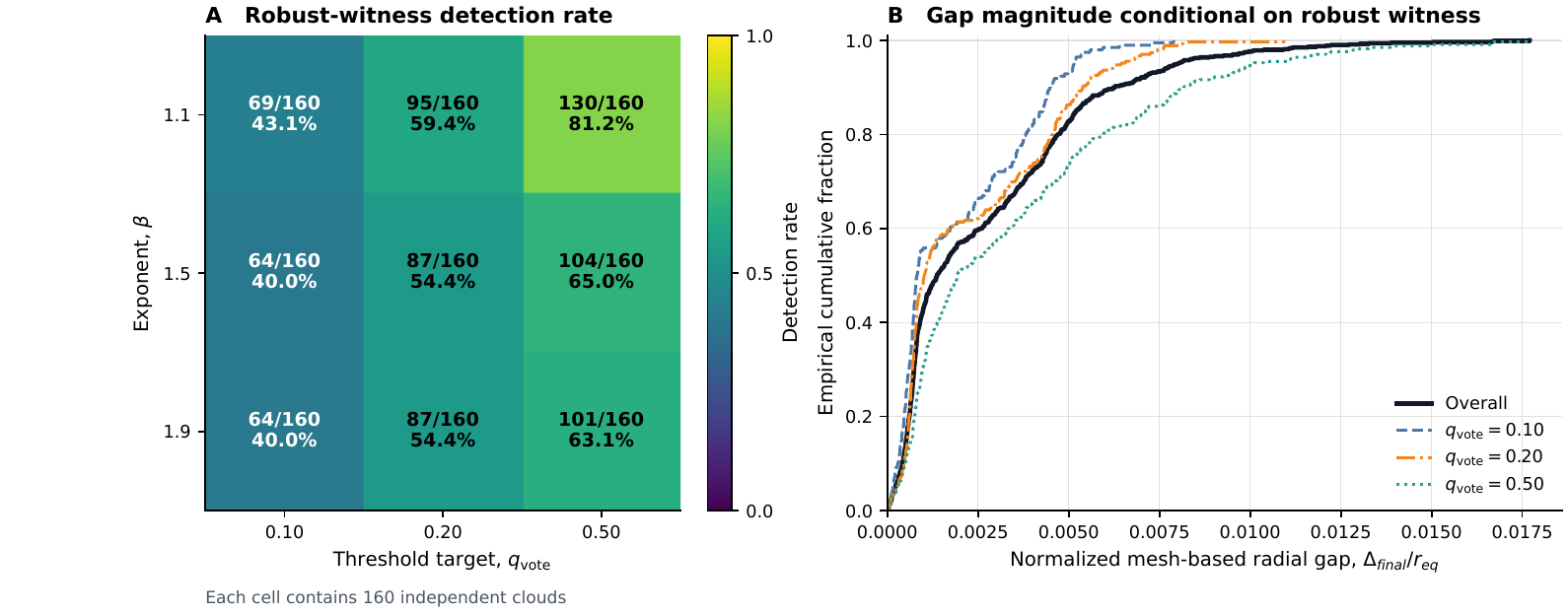These observed detection frequencies do not estimate the population prevalence of nonconvexity.

For the reported magnitude, form the metric hull $$H_M=\operatorname{conv}\{c+\widehat R_i u_i\}$$ and define the mesh-based radial convexification-gap approximation $$\widehat\Delta_{\textrm{rad}} = \max_u\left[R_{H_M}(u)-\widehat R(u)\right]_+,$$ reported after normalization by $r_{\textrm{eq}}$. Conditional on ROBUST_WITNESS, this normalized approximation had median $0.00137$, 90th percentile $0.00626$, and maximum $0.01770$. These summaries use the final gap convention. At baseline, the fallback is triggered when $\max\{|\widehat\Delta_A-\widehat\Delta_{8192}|,|\widehat\Delta_B-\widehat\Delta_{8192}|\}/r_{\textrm{eq}}>10^{-4}$ for the two interlaced 4,096-direction submeshes; the nested 16,384-direction refinement is then automatic, and its normalized 8,192-versus-16,384 discrepancy is checked against the same threshold. Exactly three cases triggered this fallback and none remained unresolved; Appendix D gives the frozen rule. In this staged numerical study, nonconvexity was frequently detectable, while its normalized radial magnitude was typically small.

Post-review Monte Carlo uncertainty summaries from the frozen outputs. No simulation was rerun. A deterministic design-stratified cloud bootstrap uses only the frozen certificate and analysis CSVs: within each of the eight $(m,\mathrm{DGP})$ strata, cloud IDs are sorted and 20 whole clouds are resampled with replacement, retaining all their $\beta/q_{\textrm{vote}}$ rows. With numpy.random.default_rng(20261001) and 20,000 replicates, the same cloud resample computes all requested summaries in each replicate and preserves the balanced 20-per-stratum design. The 2.5th and 97.5th percentiles for the median $\widetilde L/L_{\textrm{old}}$ are $[0.96380,0.96909]$ overall, $[0.93904,0.94371]$ for $m=10$, and $[0.97457,0.97609]$ for $m=25$. Table 1 gives the detection-fraction limits. These quantify finite Monte Carlo resolution of the fixed staged design; they are not population prevalence or coverage confidence intervals and imply no formal sample-size sufficiency or power claim.

7 Computational Scope and Endpoint Limitations

Theorem 2 and Corollary 3 reduce global certification to certified values on a finite directional set and a sphere-covering radius. For chord-metric covering of $\mathbb S^{d-1}$, the fixed-dimension small-radius law is $$N_d(h)=\Theta_d\!\left(h^{-(d-1)}\right), \qquad h\downarrow0,$$ consistent with standard spherical covering and packing exponents (Bhattacharya et al., 2022). If a target radial-envelope width $\tau$ satisfies $\tau>\delta$ and $\widetilde L>0$, the deterministic bound $$\delta+2\widetilde Lh\le\tau$$ is guaranteed whenever $$h\le\frac{\tau-\delta}{2\widetilde L}.$$ Consequently, for fixed $d$ and fine resolution, $$N_d = \Theta_d\!\left[ \left(\frac{2\widetilde L}{\tau-\delta}\right)^{d-1} \right].$$ If $\widetilde L=0$, the certified width is already at most $\delta$. This fixed-$d$ notation is not a dimension-growth statement; for fixed small $h$, $$\log N_d(h) = (d-1)\log(1/h)+O(d).$$ The directional burden is therefore a substantive limitation and confines the intended certification regime to low-dimensional multivariate outputs.

The endpoint $\beta=1$ separates exact geometry from unconditional certification. Corollary 1 and Theorem 1 still give common-center star-shaped geometry, but the global radial function need not be continuous or Lipschitz; Appendix A gives the exact segment example. Proposition 2 is therefore stated unconditionally only for $1<\beta<2$. At the separate degeneracy $m=1$, $I_1=\mathbb R^d$, so finite power-distance radial reconstruction begins at $m\ge2$.

The upper restriction $\beta<2$ also keeps the certified development within the strictly proper range of the conventional energy score, but the deterministic and scoring-rule roles should not be conflated. Convex comparison geometry holds for every $\beta\ge1$, including $\beta\ge2$; strict propriety has the separate boundaries summarized in Section 3. Adaptive response-dependent partition issues remain outside scope, and the paper makes no new coverage theorem or runtime-superiority claim.

The numerical assessment is limited to $d=2$, four prespecified DGPs, and a finite $\beta/q_{\textrm{vote}}$ grid. NONE_DETECTED does not certify convexity, the observed detection frequencies are not prevalence estimates, and the finite-grid secant statistic is only a lower proxy for the true Lipschitz constant.

8 Discussion

The statistical distinction driving the paper is between validity of an exact conformal set and faithful representation of that set. Standard conformal theory supplies the former. For the energy-form score studied here, the paper supplies the latter structure: exact leave-one-out comparisons become pairwise-dissimilarity sublevel sets with a common center, and convexity of those comparison sets makes the nontrivial vote aggregate star-shaped without forcing it to be convex. The univariate empirical-CRPS interval result is one specialization of this mechanism, while the analytic example shows why convexification can change the exact accepted set even when inherited coverage validity is not in question.

For $1<\beta<2$, the star-shaped geometry also supports deterministic reconstruction guarantees. Explicit radial regularity turns finite directional brackets into global radial and Hausdorff certificates, with the formal dominance $\widetilde L\le L_{\textrm{old}}$ preserved. In the frozen numerical study the median certificate tightening was approximately $3.4\%$: systematic but modest, with both certificates remaining roughly two orders above the finite-grid lower proxy and hence substantial residual certificate slack. Robust nonconvexity witnesses were often detected but typically shallow in normalized radial magnitude. These observations are descriptive for the frozen staged two-dimensional designs.

The analytic example is a stress-test and existence illustration of materially nonfaithful convexification, not a representative-magnitude claim. At the smaller observed numerical gaps, convexification may be negligible for coarse visualization or coarse summaries, while exact boundary-near candidate membership can still change. The results remain score-specific, low-dimensional, and separate from adaptive-partition coverage questions or runtime claims.

These results concern response-only energy-form FullCP. In regression-based FullCP with candidate-dependent refitting, the trial response can alter the fitted predictor and hence the score comparisons, so the common-center reduction proved here does not automatically extend to that setting. Characterizing analogous geometry under fitted-model constructions is outside the present scope.

A Exact $\beta=1$ Segment Pathology

Let $d\ge2$, $m=3$, and $$y_1=-e_1, \qquad y_2=0, \qquad y_3=e_1, \qquad \beta=1.$$ Take $$k=3,$$ which is equivalent under the strict convention to $$\frac34\le\varepsilon<1.$$ Since all three comparison votes are required, $$\Gamma^\varepsilon=I_1\cap I_2\cap I_3.$$ The middle comparison region is $$I_2 = \left\{ t:\lVert t+e_1\rVert +\lVert t-e_1\rVert \le2 \right\}.$$ By the triangle inequality, $$\lVert t+e_1\rVert +\lVert t-e_1\rVert \ge\lVert 2e_1\rVert =2,$$ and equality holds precisely on the segment joining the two foci. Hence $$I_2=[-e_1,e_1].$$ For $t=se_1$ with $-1\le s\le1$, $$\lVert t\rVert +\lVert t-e_1\rVert \le3, \qquad \lVert t\rVert +\lVert t+e_1\rVert \le3,$$ so the whole segment also lies in $I_1$ and $I_3$. Therefore $$\Gamma^\varepsilon=[-e_1,e_1].$$

The Fréchet objective is minimized at $c=0$. About this common center, $$R_\varepsilon(e_1)=R_\varepsilon(-e_1)=1,$$ whereas for every direction $u$ not collinear with $e_1$ the ray $\{ru:r>0\}$ leaves the segment immediately, so $$R_\varepsilon(u)=0.$$ Thus the radial function is discontinuous on $\mathbb S^{d-1}$ when $d\ge2$. Exact common-center star-shaped geometry at $\beta=1$ therefore does not imply an unconditional global Lipschitz radial certificate.

B A Three-Point Nonconvex Robustness Witness

Consider $$d=2, \qquad m=3, \qquad \beta=\frac32,$$ $$y_1=(-1,0), \qquad y_2=(1,0), \qquad y_3=(0,1.5),$$ and $$\varepsilon=0.6, \qquad k=2.$$ A common Fréchet minimizer is $$c=(0,0.5247333004905787534\ldots).$$ Let $$A=(0.58,-0.94), \qquad B=(-0.58,-0.94), \qquad M=(0,-0.94).$$ For $G_j(t)=\sum_{i\ne j}\lVert t-y_i\rVert ^{3/2}$ and the corresponding $d_j$, the resulting comparison margins and vote counts are $$\begin{array}{c|rrr|c} & d_1-G_1 & d_2-G_2 & d_3-G_3 & N(\cdot)\\ \hline A& +0.232492290498& -1.215637558202& +1.303611687945& 2\\ B& -1.215637558202& +0.232492290498& +1.303611687945& 2\\ M& -0.170268407563& -0.170268407563& +1.625412619066& 1 \end{array}$$ Because $k=2$ and equality would count as a vote, these strict numerical margins imply $$A,B\in\Gamma^\varepsilon, \qquad M\notin\Gamma^\varepsilon.$$ The witness therefore supplies an accepted-endpoints/rejected-midpoint nonconvexity check with nonzero margins.

C Technical Proof Details

For a non-singleton comparison set $I_j$, let finite positive constants $V_{ij}$ satisfy $$\sup_{t\in I_j}\lVert t-y_i\rVert \le V_{ij}, \qquad i\ne j,$$ and define $$M_j(V)=\beta\sum_{i\ne j}V_{ij}^{\beta-1}, \qquad \lambda_j(V)=\beta(\beta-1)\sum_{i\ne j}V_{ij}^{\beta-2}.$$ The calculations below prove the modular bound $$\operatorname{Lip}(R_j)\le\frac{2M_j(V)}{\lambda_j(V)}.$$ The explicit main-text choice is $V_{ij}=U_{ij}$; singleton comparison sets are handled by the constant-zero radial argument.

This appendix is the unique detailed location for the technical calculations underlying Section 5.

References

- Arnau, R., Calabuig, J. M., Erdoğan, E., & Sánchez Pérez, E. A. (2023). Extension procedures for lattice Lipschitz operators on Euclidean spaces. Revista de La Real Academia de Ciencias Exactas, Físicas y Naturales. Serie A. Matemáticas, 117(2). https://doi.org/10.1007/s13398-023-01402-0 ↩ 1 2
- Balashov, M. V., & Golubev, M. O. (2012). About the Lipschitz property of the metric projection in the Hilbert space. Journal of Mathematical Analysis and Applications, 394(2), 545–551. https://doi.org/10.1016/j.jmaa.2012.05.024 ↩
- Bhattacharya, A., Freund, Y., & Jaiswal, R. (2022). On the k-means/median cost function. Information Processing Letters, 177, 106252. https://doi.org/10.1016/j.ipl.2022.106252 ↩
- Diquigiovanni, J., Fontana, M., & Vantini, S. (2022). Conformal prediction bands for multivariate functional data. Journal of Multivariate Analysis, 189, 104879. https://doi.org/10.1016/j.jmva.2021.104879 ↩
- Gan, F., & Liu, Y. (2025). Conformal prediction for multivariate responses with Euclidean likelihood. Journal of Multivariate Analysis, 210, 105494. https://doi.org/10.1016/j.jmva.2025.105494 ↩
- Gneiting, T., & Raftery, A. E. (2007). Strictly Proper Scoring Rules, Prediction, and Estimation. Journal of the American Statistical Association, 102(477), 359–378. https://doi.org/10.1198/016214506000001437 ↩ 1 2
- Johnstone, C., & Ndiaye, E. (2025). Exact and approximate conformal inference for multi-output regression. Proceedings of the Fourteenth Symposium on Conformal and Probabilistic Prediction with Applications, Proceedings of Machine Learning Research, 266, 153–172. ↩ 1 2 3
- Lei, J., G’Sell, M., Rinaldo, A., Tibshirani, R. J., & Wasserman, L. (2018). Distribution-Free Predictive Inference for Regression. Journal of the American Statistical Association, 113(523), 1094–1111. https://doi.org/10.1080/01621459.2017.1307116 ↩
- Ndiaye, E., & Takeuchi, I. (2023). Root-finding approaches for computing conformal prediction set. Machine Learning, 112(1), 151–176. https://doi.org/10.1007/s10994-022-06233-5 ↩ 1 2
- Razafindrakoto, D. L., Celisse, A., & Lacaille, J. (2026a). Approximate full-conformal multi-task regression with reproducing kernels. https://arxiv.org/abs/2607.00645
- Razafindrakoto, D. L., Celisse, A., & Lacaille, J. (2026b). Approximate full-conformal prediction in an RKHS. https://arxiv.org/abs/2601.13102
- Shafer, G., & Vovk, V. (2008). A tutorial on conformal prediction. Journal of Machine Learning Research, 9(12), 371–421. ↩ 1 2
- Toccaceli, P. (2026). CRPS-optimal binning for univariate conformal regression. https://arxiv.org/abs/2603.22000
- Vovk, V., Gammerman, A., & Shafer, G. (2005). Algorithmic learning in a random world. Springer. https://doi.org/10.1007/b106715 ↩
Cite this article
Feng, Y. (2026). Common-Center Geometry and Certified Radial Reconstruction for Energy-Form Full Conformal Regions. Journal of Reproducible Statistics, 1, 6. https://doi.org/10.68365/jrepstat.2026.6
Feng, Yiheng. 2026. “Common-Center Geometry and Certified Radial Reconstruction for Energy-Form Full Conformal Regions.” Journal of Reproducible Statistics 1: 6. https://doi.org/10.68365/jrepstat.2026.6.
Feng Y. Common-Center Geometry and Certified Radial Reconstruction for Energy-Form Full Conformal Regions. Journal of Reproducible Statistics. 2026;1:6. doi:10.68365/jrepstat.2026.6
Feng, Y. (2026) “Common-Center Geometry and Certified Radial Reconstruction for Energy-Form Full Conformal Regions,” Journal of Reproducible Statistics, 1, p. 6. Available at: https://doi.org/10.68365/jrepstat.2026.6.
doi: https://doi.org/10.68365/jrepstat.2026.6
Downloads
https://doi.org/10.68365/jrepstat.2026.6 also supports content negotiation, so reference managers can fetch the citation from the DOI directly. The exports above work without it.