The Constrained LASSO is a Portfolio: A numerical check of the CLA–LASSO identity under constraints

Thomas Schmelzer

doi:10.68365/jrepstat.2026.10

Research article · Published 2026-11-01 · Open access, CC-BY 4.0

The Constrained LASSO is a Portfolio: A numerical check of the CLA–LASSO identity under constraints

Thomas Schmelzer¹

¹ Jebel Quant Research, Abu Dhabi · orcid 0009-0009-9771-3501

constrained LASSOcritical line algorithmsolution pathcompositional dataportfolio optimisationreproducibility

doi: https://doi.org/10.68365/jrepstat.2026.10 Vol. 1 (2026) · Art. 10 Version 1 how to cite ↓ html pdf (typeset)

✓ Reproduced

Reproducibility record

verified 2026-10-26

Result: Reported results reproduced. All counts, declines and certificates reproduce on macOS arm64 and Linux. Near interpolating fits two residual bounds are exceeded, one of them 14-fold.; ✓ measured
Entry point: cd code/lasso-327bcd7a798d51e8a92ac6babdfb8ede62ef1e42/preprints/constrained_lasso && make reproduce; ✓ executed
Environment: Python 3.12 from the lockfiles via uv, Julia 1.12.6, R 4.6.1 with Rglpk 0.6.5.1, Linux aarch64 container and macOS arm64; ✓ measured
Determinism: Seeded.; declared
Archive: the-constrained-lasso-is-a-portfolio-a-numerical-check-of-the-cla-lasso-identity-under-constraints-v1-repro.zip · reviewed bundle SHA-256 17fde9d45a841795b52d55cc99ce5585bfde3b78d31a540d4bfa2a6aea389552 · https://doi.org/10.5281/zenodo.23863450; ✓ computed
Code: https://github.com/Jebel-Quant/lasso/tree/main/preprints/constrained_lasso; declared
Data: Open.; declared, route checked

Reproducibility package (.zip, 10.4 MB) · Zenodo doi:10.5281/zenodo.23863450 · SHA-256 da774fd9a0c99c4755bb1ff8c865bae1b4091f5979caff4cc48b25791e2f0e01

$cd code/lasso-327bcd7a798d51e8a92ac6babdfb8ede62ef1e42/preprints/constrained_lasso && make reproduce

Reproduce: cd code/lasso-327bcd7a798d51e8a92ac6babdfb8ede62ef1e42/preprints/constrained_lasso && make reproduce · code & data via doi:10.68365/jrepstat.2026.10

Open review

Peer review record

2 rounds · 3 reviewers · signed Full reviewsHide reviews 2026-10-26Minor revision2026-10-264 answers2026-10-26Accepted

The decision letters, the reports the authors read, their answers and the editor's signed decisions, as written. The reports come from the journal's review engine. The authors could have kept this record private until they confirmed the proof.

Round 1Minor revision3 reviewers · response

Minor revisionConfirmed and signed by Matthias Templ2026-10-26 · orcid 0000-0002-8638-5276

Decision letter2026-10-26This note verifies numerically that a released portfolio Critical Line Algorithm, wrapped in two thin encodings, computes exact constrained-LASSO solution paths across caps, signs, equality and inequality rows, zero sums and monotone fits, matching LARS, an interior-point solver and three independent path algorithms to rounding, including when there are more predictors than observations. It matters to practitioners who need constrained-LASSO paths that lars_path cannot produce, and to portfolio and statistics readers who can now use one active-set solver across both problems. The reviewers found nothing to fix in the writing itself. We would be glad to see the revised version.

Thank you for your submission to JRepStat. We are inviting a minor revision. The reviewers’ points follow, grouped by weight.

This note verifies numerically that a released portfolio Critical Line Algorithm, wrapped in two thin encodings, computes exact constrained-LASSO solution paths across caps, signs, equality and inequality rows, zero sums and monotone fits, matching LARS, an interior-point solver and three independent path algorithms to rounding, including when there are more predictors than observations. It matters to practitioners who need constrained-LASSO paths that lars_path cannot produce, and to portfolio and statistics readers who can now use one active-set solver across both problems. The reviewers found nothing to fix in the writing itself. We would be glad to see the revised version.

How to read this letter. The decision rests on the items marked required. If a required item seems wrong to you, or cannot be done within this paper, decline it on the revision page and give the reason. A reasoned decline is a legitimate answer, and the editor weighs it. Reviewers can be mistaken. Items marked recommended or optional are advice from the reviewers. Adopt them, decline them with a sentence, or leave them for later work. None of that counts against the paper. The reviewer reports below carry the same marks. The editor who signs this decision may weigh an item differently in the accompanying message, and that message prevails.

required (the decision rests on these):

[Reviewer 2] State the exact objective of the linear program behind the KKT certificate, so a reader can see that a small reported value certifies optimality.
[Reviewer 3] State that the random designs use fixed seeds recorded in the repository, and add a short determinism attestation: on a fixed platform the discrete outputs (knot counts, which problems are declined, certificate pass or fail) reproduce exactly, while near-rounding residuals vary only in the last digits. Table 4 and Table 5 report knot counts as ranges over three seeds, so the exact figures the text quotes depend on the seeds being pinned.

recommended:

[visualisation] Figure 3 distinguishes its eight largest genera by colour alone against grey, with no direct line labels. Eight categorical hues are hard to separate under common forms of colour vision deficiency. Draw the eight from a colourblind-safe qualitative palette and label each line at its right-hand end, so the series read without reliance on hue.
[visualisation] The penalty axis in Figures 1 and 3 reads “0 10^1 10^2” with λ decreasing, which looks like a reversed symlog axis. State the axis transform in the caption (symlog with its linear threshold, reversed) so a reader can place the knots; the units (λ) are labelled, scales are not truncated to exaggerate, and the shaded “beyond the cap” bands in Figure 1 are an honest way to mark the constraint.
[software-landscape] A single feature table listing which constraint types each package accepts (caps, per-coefficient signs, equality rows, inequality rows, zero sums, p>n, ridge-free) would consolidate what is now spread across Sections 5.5, 5.6 and the related-work paragraph, and would make the placement against comlasso, c-lasso and Gaines et al. legible at a glance. The paper stands without it.
[Reviewer 1] The diabetes motivating example reads as a modeling endorsement; frame it as an illustration, note the cap u is chosen post hoc, and separate the “low HDL is a risk factor” claim (which [20] supports for incident diabetes) from the inference about disease progression (the outcome here).
[Reviewer 1] The runtime comparison in Section 5.3 is only against a grid of interior-point solves; add a note on runtime versus the dedicated path algorithms (comlasso, Gaines et al., c-lasso), or state why a cross-language timing is not comparable, so the “when to use it” guidance is complete.
[Reviewer 1] The “sum to one” example is described “as a synthetic control does”, but classic synthetic control also constrains weights to be nonnegative; clarify that this is a negative-weight variant so the analogy is not misread.
[Reviewer 1] State that the sCD14 and other real-data paths are computational demonstrations and that no biological inference is intended.
[Reviewer 2] Name the single published test whose path fails the segment check and report what the check returns there.
[Reviewer 2] Report the hostile and scale tables over more than three seeds, keeping the worst case.
[Reviewer 2] State the relaxation values of epsilon and note that the certificate, not the extrapolation, guarantees the returned path.
[Reviewer 2] Clarify how the gap against LARS is read where the minimiser may not be unique, and which five of the Table 2 problems the ported Gaines algorithm matches.
[Reviewer 3] Document the R toolchain that executes comlasso 0.2. The text says R 4 will not install a package built for R 3, then says the check loads it unchanged, which leaves unclear which R interpreter runs the comparison and whether a package built for R 3 behaves identically when sourced under a later R.
[Reviewer 3] Report the timing methodology behind the cost ratios in Section 5.3 (number of runs and the spread), instead of “the fastest of several runs”.
[Reviewer 3] Provide a mirror or archival fallback for the sCD14 source (coda4microbiome 0.2.4), since the fetch depends on CRAN retaining that version; the SHA-256 check confirms identity but not availability.

optional:

[statistical-rigor] The simulated and hostile-problem claims rest on three seeds each with worst-case reporting (Tables 4 and 5). Worst-of-three is a conservative summary and no claim depends on a sampling distribution, so this is adequate for the paper’s purpose. A larger seed count would let the dependence of the gap on conditioning be characterised as a distribution rather than a single worst case, if a later paper wanted that.
[Reviewer 1] A predictive comparison (for example cross-validation) showing the constrained fits generalise would strengthen the applied case, though it is beyond the scope of this note.

Reviews

Report Reviewer 1recommends acceptThis is a verification note, and judged as one it does its job well. The underlying identity between the constrained LASSO path and the CLA path is proven elsewhere [14]; the work here is to show that a portfolio solver, through two encodings (Propositions 1 and 2), actually reproduces the constrained-LASSO knots on a wide spread of constraint types, and to check every path against references that know nothing of portfolios. The test matrix is the strength of the paper. Caps, signs, equality rows, inequality rows, zero sums, monotone orderings, a pinned observation and a sum-to-one constraint are each exercised, on simulated and real data, with LARS as the knot-by-knot reference where it applies and an interior-point solve at segment midpoints elsewhere, backed by a direct optimality check that holds along whole segments rather than only at midpoints. The agreement is at the level of rounding. The hostile cases (near-duplicate columns, correlation 0.99999, p>n with a zero sum) and the deliberate decline of the 1e-6 duplicate are the kind of adversarial testing I want to see in a paper whose whole claim is numerical. The honesty about where references add a ridge, and the point that the CLA needs none for p>n, is both correct and genuinely useful to someone choosing a tool for microbiome-scale zero-sum problems.

Written by the journal's review engine in the role of the application reviewer, and read by the editor before the decision. How the engine works is on the peer review page.

This is a verification note, and judged as one it does its job well. The underlying identity between the constrained LASSO path and the CLA path is proven elsewhere [14]; the work here is to show that a portfolio solver, through two encodings (Propositions 1 and 2), actually reproduces the constrained-LASSO knots on a wide spread of constraint types, and to check every path against references that know nothing of portfolios. The test matrix is the strength of the paper. Caps, signs, equality rows, inequality rows, zero sums, monotone orderings, a pinned observation and a sum-to-one constraint are each exercised, on simulated and real data, with LARS as the knot-by-knot reference where it applies and an interior-point solve at segment midpoints elsewhere, backed by a direct optimality check that holds along whole segments rather than only at midpoints. The agreement is at the level of rounding. The hostile cases (near-duplicate columns, correlation 0.99999, p>n with a zero sum) and the deliberate decline of the 1e-6 duplicate are the kind of adversarial testing I want to see in a paper whose whole claim is numerical. The honesty about where references add a ridge, and the point that the CLA needs none for p>n, is both correct and genuinely useful to someone choosing a tool for microbiome-scale zero-sum problems.

My concerns are about the applied framing, not the computation. The opening diabetes example is doing a lot of rhetorical work in Section 1 and Figure 1, and an applied reader may take it as a claim that the capped fit is the better model of the biology. The cap value u = 396.1 is chosen as half the largest least-squares coefficient, which is a post hoc choice, and the robustness sentence (caps up to 637 keep HDL negative) is reassuring but still conditional on this dataset. Separately, the reference [20] supports low HDL as a risk factor for incident diabetes, whereas the response in this dataset is a continuous measure of disease progression. The sign argument slides between those two outcomes. The cleanest fix is to present the example as an illustration of what a cap does to offsetting coefficients, and to qualify the biological reading as suggestive.

On guidance to users, the cost comparison in Section 5.3 is careful and precise, but it compares only against a grid of interior-point solves. The paper also runs comlasso, the Gaines et al. algorithm and c-lasso for accuracy, so a reader deciding between tools will want to know how the CLA compares to those on runtime, not only to an IPM grid. A single paragraph, even one that explains why a fair cross-language timing is not available, would round out the “when to use it” section. The “sum to one” example invokes synthetic control, and since the classic synthetic control estimator also constrains weights to be nonnegative, a one-line clarification that this is the negative-weight variant will stop the analogy being over-read. Finally, the sCD14 path is a good stress test on real compositional data, and a sentence stating that it is a computational demonstration with no biological conclusion attached will keep it from being cited as a finding about inflammation.

The reproducibility posture is strong as described: lockfiles pinning Python 3.12 and package hashes, a single script that writes every number quoted in the text, pinned and checksummed R and Julia environments, a checksum on the fetched sCD14 data that is not redistributed, and a stated tolerance regime that accounts for hardware-dependent last digits. I did not execute the artifacts in this pass, so I assess them as declared and leave the run itself to the reproducibility lens. None of the items below blocks acceptance; they improve how an applied reader will receive the paper.

Numbered suggestions to the authors:

recommended Reframe the diabetes example in Section 1 and Figure 1 as an illustration of what the cap does to offsetting coefficients. State that u = 396.1 is chosen after seeing the least-squares fit, and separate the HDL risk-factor claim (which [20] supports for incident diabetes) from the inference about progression, which is this dataset’s outcome.
recommended In Section 5.3 and the “when to use it” discussion, add how the CLA compares on runtime to the dedicated path algorithms you already run (comlasso, Gaines et al., c-lasso), or state why a fair cross-language timing is not available, so the cost guidance is not read as comparing only against an IPM grid.
recommended Clarify in Section 5.1 that the “sum to one” example allows negative weights, unlike the classic synthetic control estimator, so the synthetic-control analogy is not misread.
recommended Add a sentence where sCD14 is introduced stating that it and the other real-data paths are computational demonstrations and that no biological inference is intended.
optional A predictive comparison, such as cross-validation of the constrained versus unconstrained fits, would strengthen the applied argument that constraints buy interpretability without cost, though it sits beyond the scope of this note.

Report Reviewer 2recommends minorThis is a validation note with a clear and narrow job. A theoretical identity between the constrained LASSO path and the Critical Line Algorithm path is proved elsewhere [14]. Here the author poses constrained regressions as portfolios through two encodings, runs them through a released portfolio CLA, and asks whether the resulting paths match independent references. The question is well posed and the design answers it in the right way. The two encodings in Propositions 1 and 2 are stated cleanly and their proofs are correct as given. The split into nonnegative long and short parts, the simplex rescaling with a riskless asset, and the multiplier bookkeeping all follow from the classical bound-penalty equivalence, and the paper is careful to say that the propositions borrow nothing from [14] beyond that equivalence.

Written by the journal's review engine in the role of the methodology reviewer, and read by the editor before the decision. How the engine works is on the peer review page.

This is a validation note with a clear and narrow job. A theoretical identity between the constrained LASSO path and the Critical Line Algorithm path is proved elsewhere [14]. Here the author poses constrained regressions as portfolios through two encodings, runs them through a released portfolio CLA, and asks whether the resulting paths match independent references. The question is well posed and the design answers it in the right way. The two encodings in Propositions 1 and 2 are stated cleanly and their proofs are correct as given. The split into nonnegative long and short parts, the simplex rescaling with a riskless asset, and the multiplier bookkeeping all follow from the classical bound-penalty equivalence, and the paper is careful to say that the propositions borrow nothing from [14] beyond that equivalence.

The strongest methodological choice is the optimality certificate. Comparing a path only against another numerical solver bounds the error at the solver’s own tolerance, and the paper says so. Evaluating the subgradient conditions of problem (1) directly, at every knot and across every whole segment, with the multipliers chosen by a linear program and the residual then evaluated exactly, removes that ceiling. Checking the segment whole rather than at its midpoint alone is the right refinement, since a path can be right at both ends and at the midpoint and still cut across a knot. This is where I want one more sentence. The certificate’s force rests on what the linear program optimises. The text says the multipliers are chosen to “satisfy the conditions best”, which a reader cannot pin down. If the program minimises the largest violation across all the conditions jointly, subject to the sign constraint on the active-row multipliers, then a small reported value is a genuine optimality certificate and a true violation cannot be hidden. Please state that objective explicitly, because the whole evidential weight of the paper sits on it.

Two further points concern how much a reader can trust the stress results. The hostile and scale tables are drawn with three seeds and report the worst case. Three draws is thin for a claim that an algorithm declines or stays exact on a whole family of ill-conditioned designs. Re-running over more seeds and keeping the worst would make the boundary between “traced exactly” and “declined” look stable rather than incidental. Relatedly, the text claims that one of the published tests contains a path that fails the segment check, which would be a welcome demonstration that the check has teeth. I could not locate which test this is or what the check reports there. Naming it and giving its residual would turn an assertion about the check into evidence for it.

The treatment of degenerate starts is handled honestly as an implementation device, with an extrapolation in epsilon and a certificate afterwards. Because the extrapolation is a two-point Richardson step and its affineness “cannot be checked in advance”, the reader should be told which epsilon values are used and reminded that the returned path is guarded by the certificate and not by the extrapolation itself. On uniqueness, the paper is appropriately cautious, testing optimality and not uniqueness where p exceeds n. One consequence deserves a line. Where the minimiser is not unique, LARS and the CLA may trace different paths of minimisers, so a gap against LARS is not by itself a defect. The hostile section already argues “both paths are right” from the conditioning bound, and a short statement folding that logic into the non-unique case, together with naming which five Table 2 problems the ported Gaines algorithm matches, would close the remaining ambiguity.

On reproducibility I can only review what is declared, since the scripts were not provided to run in this pass. As declared the artifacts are unusually complete: lockfiles with versions and hashes, a single script that writes every quoted number, a checksummed download of the microbiome data, legacy R and Julia references pinned and ported with departures marked, and CI. This is the standard a validation paper should meet, and it is met on paper. The competing-interests statement is precise about what the author wrote and what the references are. None of the above changes the paper’s conclusion, which the evidence supports. The asks are about letting a reader verify the certificate and the stress claims with the same confidence the author has.

Numbered suggestions to the authors:

required State the exact objective of the linear program used in the optimality check, specifically that it minimises the largest violation across the KKT conditions of (1) jointly, under the nonnegativity constraint on the active-row multipliers, so that a small reported value certifies optimality and a real violation cannot be masked.
recommended Name the one published test whose path fails the segment check, and report what the check returns there, so the check’s discriminating power is shown rather than asserted.
recommended Re-run the hostile problems of Table 4 and the scale problems of Table 3 over more than three seeds, keeping the worst case, so the line between “traced exactly” and “declined” reads as stable.
recommended Give the relaxation values of epsilon used for degenerate starts and add one sentence that the certificate, not the two-point extrapolation, guarantees the returned path.
recommended Add a sentence on how the gap against LARS is interpreted where the minimiser need not be unique, and name which five of the Table 2 problems the ported Gaines algorithm matches when started at the exact first knot.

Report Reviewer 3recommends minorThis is a reproducibility-first paper, and on that axis it is well built. There is a single entry point (make figures) that computes every path, runs every check, and writes every figure, table and quoted number, so the text and the code cannot drift apart silently. The environment is captured with lockfiles that pin Python 3.12 and every package by version and hash, the cross-language checks are pinned (Julia 1.12, a checksummed comlasso commit, c-lasso 1.0.11), and the whole thing runs in CI. The non-redistributable sCD14 data are fetched with a SHA-256 check rather than shipped. The competing-interests statement is clear about the author maintaining cvxcla and separates that from the external references. The hardware caveat is handled honestly: residuals near rounding differ in the last digits across CPUs, tolerances are set between 1e-12 and 1e-10, and timings are given only as ratios. This is close to what I would want from a numerical-check submission.

Written by the journal's review engine in the role of the software reviewer, and read by the editor before the decision. How the engine works is on the peer review page.

This is a reproducibility-first paper, and on that axis it is well built. There is a single entry point (make figures) that computes every path, runs every check, and writes every figure, table and quoted number, so the text and the code cannot drift apart silently. The environment is captured with lockfiles that pin Python 3.12 and every package by version and hash, the cross-language checks are pinned (Julia 1.12, a checksummed comlasso commit, c-lasso 1.0.11), and the whole thing runs in CI. The non-redistributable sCD14 data are fetched with a SHA-256 check rather than shipped. The competing-interests statement is clear about the author maintaining cvxcla and separates that from the external references. The hardware caveat is handled honestly: residuals near rounding differ in the last digits across CPUs, tolerances are set between 1e-12 and 1e-10, and timings are given only as ratios. This is close to what I would want from a numerical-check submission.

The gap I would close before this is treated as fully reproducible is around randomness. Tables 4 and 5 report knot counts as ranges over three seeds (for example 43–45, 92–228, 50–78), which tells me the discrete structure of the path moves with the seed. For the specific numbers in the text to be reproducible, the seeds have to be fixed and recorded in the repository, and a reader needs to know that. A short determinism statement would settle it: on a fixed platform with the recorded seeds, the knot counts, the set of declined problems, and the certificate outcomes reproduce exactly, and only the near-rounding residuals vary. The paper already supplies the hardware half of this, so the missing half is the seed and discrete-output half.

Two smaller reproducibility points concern the external checks that carry real evidential weight. The comlasso check agrees with the CLA to 4.3e-15, which is convincing, but the code-availability paragraph first says R 4 will not install a package built for R 3 and then says the check loads it unchanged. Which R runs the comparison, and how a package built for R 3 is loaded under it, should be stated so the reader can rebuild that leg of the check. Separately, the cost ratios in Section 5.3 rest on “the fastest of several runs,” which is a weak basis for a timing claim even when the claim is secondary to correctness. Reporting how many runs and the spread would make those ratios as defensible as the rest of the numbers.

On the sCD14 fetch, pinning by SHA-256 guards against the file changing but not against it disappearing from CRAN. A mirror or an archived copy, or a sentence naming a fallback, would keep that one real-data check reproducible over time. None of this touches the core correctness evidence, which is internally strong and triangulated across LARS, an interior-point solver and three independent path algorithms, with the KKT conditions evaluated along whole segments rather than at midpoints alone.

Numbered suggestions to the authors:

required Record the seeds for the random designs (Wide, Correlated, Duplicate, Monotone, Sum to one, and the simulated zero-sum problems) in the repository and say so in the paper, and add a one-sentence determinism attestation that on a fixed platform the knot counts, the declined problems and the certificate outcomes reproduce exactly while near-rounding residuals vary only in the last digits.
recommended State which R interpreter runs comlasso 0.2 and how a package built for R 3 is loaded under it, so the comlasso comparison can be rebuilt.
recommended Give the timing methodology for the cost ratios in Section 5.3 (number of runs and the spread) instead of reporting the fastest of several runs.
recommended Add a mirror or archival fallback for coda4microbiome 0.2.4 so the sCD14 check survives the CRAN version being removed.

Revision

Authors' response2026-10-26 · 4 answersAuthors confirm each required point as done or give their reason for declining it. Further answers are voluntary, because the review compares every revision with the previous version and the next round's reports say what remains open.

Authors confirm each required point as done or give their reason for declining it. Further answers are voluntary, because the review compares every revision with the previous version and the next round's reports say what remains open.

required State the exact objective of the linear program behind the KKT certificate, so a reader can see that a small reported value certifies optimality.

Done

required State that the random designs use fixed seeds recorded in the repository, and add a short determinism attestation: on a fixed platform the discrete outputs (knot counts, which problems are declined, certificate pass or fail) reproduce exactly, while near-rounding residuals vary only in the last digits. Table 4 and Table 5 report knot counts as ranges over three seeds, so the exact figures the text quotes depend on the seeds being pinned.

Done

recommended The diabetes motivating example reads as a modeling endorsement; frame it as an illustration, note the cap u is chosen post hoc, and separate the "low HDL is a risk factor" claim (which [20] supports for incident diabetes) from the inference about disease progression (the outcome here).

Done We reframed it slightly to avoid this impression

optional A predictive comparison (for example cross-validation) showing the constrained fits generalise would strengthen the applied case, though it is beyond the scope of this note.

Declined It's indeed beyond the scope of this note

The authors' full response letter (PDF)

Round 2Accepted3 reviewers

AcceptedSigned by Matthias Templ2026-10-26 · orcid 0000-0002-8638-5276

The editor's note

All three reviewers recommend acceptance. Both required points of the first round are met: Section 5.1 now states the objective of the linear program behind the optimality certificate, and the availability section records the seeds with a test that checks the discrete results. The editor accepted the final version after the journal reproduced it. One correction remains for the proof, a stray full stop in Section 5.5.

Decision letter2026-10-26Congratulations, your manuscript has been accepted for publication in JRepStat. Production begins now.

Congratulations, your manuscript has been accepted for publication in JRepStat. Production begins now.

Where it is not on file yet, we still need the following for production.

a valid ORCID iD for every author
a captured computational environment (dependencies/lockfile/container)
a signed determinism attestation for the entry-point command

Reviews

Report Reviewer 1recommends acceptOf the four recommended points and one optional point I raised, three are adopted and two are answered with a reason.

Written by the journal's review engine in the role of the application reviewer, and read by the editor before the decision. How the engine works is on the peer review page.

Of the four recommended points and one optional point I raised, three are adopted and two are answered with a reason.

The two I weighed carefully are the declines. On runtime against the dedicated path algorithms (my point 2), the paper now states in Section 6 why a cross-language timing would measure the languages and the ports rather than the algorithms, and directs the user to Table 6 to choose by the constraints each tool accepts and then to time candidates on their own problem. That is the alternative I named, and it convinces me: comlasso read under R 4, a Julia 0.6 port and a c-lasso grid with a fixed ridge are not comparable stopwatches, and a number would mislead more than it informs. On the predictive comparison (my point 5), the decline as beyond the scope of a verification note is right, and the revised framing of the diabetes and sCD14 examples removes the suggestion that any predictive claim is being made.

The applied framing I was concerned about is now clean. The diabetes example reads as an illustration of what a cap does to offsetting coefficients, with u = 396.1 marked as chosen after seeing the fit, the incident-diabetes risk-factor claim from [22] separated from the progression outcome, and the cap robustness described as a property of these data. The sum-to-one example now distinguishes itself from the nonnegative-weight synthetic control estimator, and sCD14 is labelled a computational demonstration in both the text and Figure 3.

One change the revision made in answer to another reviewer is worth noting as newly visible, since it affects how an applied reader should read the headline claim: the extra seeds moved one p>n draw of Zero-sum, signs to a worst KKT residual of 1.0×10^-9 near an interpolating fit at cond(X) ≈ 6×10^15, and the abstract and Section 5.5 now state this rather than claiming rounding-level residuals there. This is honest and correct, and it does not weaken the applied case. The paper’s claim is about where each tool’s path ends and whether it declines rather than answers wrongly, and that claim is now stated with the right precision.

I recommend acceptance.

Numbered suggestions to the authors:

(none open)

Report Reviewer 2recommends acceptOf the one required point and four recommended ones I raised, all are met.

Written by the journal's review engine in the role of the methodology reviewer, and read by the editor before the decision. How the engine works is on the peer review page.

Of the one required point and four recommended ones I raised, all are met.

The required point, the objective of the linear program behind the KKT certificate, is now stated in Section 5.1 at the level the evidential weight demands: the program minimises a single number, the largest violation across the optimality conditions of (1) taken jointly under the nonnegativity constraint on the active-row multipliers, with the violation re-evaluated exactly at the multipliers found. The reader can now see why a small reported value certifies optimality to that size and why a real violation cannot be masked. This closes the one point the decision rested on.

The re-run over more seeds did more than tighten a table. Extending Table 3 to three seeds, Tables 4 and 5 to ten, and keeping the worst case moved the boundary between “traced exactly” and “declined”, and it exposed three further defects in cvxcla 2.7.0, two in the segment-optimality check and one in the plain homotopy, now fixed in 2.7.1 with regression tests and reported in Section 1 alongside the earlier two. The paper no longer claims rounding-level residuals where a p > n path nears an interpolating fit, and the abstract and Section 5.5 now carry the 10^-9 figure. This is the right outcome of the ask, and the reporting of it is accurate to what the seeds showed.

The remaining three are settled. The segment check now names test_segment_check_sees_between_samples and gives both numbers, the exact optimality residual of zero at the ends and the midpoint against the 0.25 the segment check returns, which demonstrates the check has teeth. The epsilon relaxation schedule (10^-6, 10^-7, 10^-8 times the coefficient scale) is stated in Section 4 with the sentence separating what the extrapolation proposes from what the certificate guarantees. The non-uniqueness reading is folded into Sections 5.4 and 5.6, and the five Table 2 problems the ported Gaines algorithm matches at the exact first knot are named. One production-level item remains for the proof, a stray full stop in Section 5.5.

Numbered suggestions to the authors:

[editor_fix] In Section 5.5, join “with cond(X) near 10^16. and the interior-point solver agrees to 4.2×10^-6” into one sentence, removing the stray full stop before “and”.

Report Reviewer 3recommends acceptThe required point is settled. The seeds are now recorded in python/make_figures.py (seed 7 for Table 2, 7–9 for Table 3, 7–16 for Tables 4 and 5), the determinism attestation is in the Code and data availability section, and test_deterministic runs the Table 3 and Table 4 problems twice and asserts the discrete outputs match. That closes the gap I flagged: the knot counts, the declined problems and the certificate outcomes are now pinned, and the text says which digits are allowed to move.

Written by the journal's review engine in the role of the software reviewer, and read by the editor before the decision. How the engine works is on the peer review page.

The required point is settled. The seeds are now recorded in python/make_figures.py (seed 7 for Table 2, 7–9 for Table 3, 7–16 for Tables 4 and 5), the determinism attestation is in the Code and data availability section, and test_deterministic runs the Table 3 and Table 4 problems twice and asserts the discrete outputs match. That closes the gap I flagged: the knot counts, the declined problems and the certificate outcomes are now pinned, and the text says which digits are allowed to move.

My three recommended points are also met. The comlasso leg now states R 4.6.1 runs the check and that the R 3.2 package is read with lazyLoad from serialized code at a pinned, checksummed commit, with the point that comlasso carries no compiled code, so the loading path is reconstructible. Section 5.3 gives the timing methodology (warm-up run, then 11 timed runs, 3 at the largest size, ratio of medians with the paired-run spread within 8%). The sCD14 fetch now falls back from CRAN to the CRAN archive to a dated Posit snapshot, with the tarball digest pinned per source and the inner data file checked byte for byte, so the real-data check survives a CRAN version removal.

One thing worth recording for the editor rather than the author: the extra seeds the author drew in response to another reviewer surfaced three defects in cvxcla 2.7.0 and shifted the boundary between traced and declined (Duplicate 10⁻⁶ under the cap now declined on 2 of 10 seeds, and a worst-case p>n residual of 1.0×10⁻⁹). The revision reports all of this in the text and the abstract rather than smoothing it over, and the fixes ship in 2.7.1 with regression tests. From the reproducibility angle this strengthens the paper, since the released version now matches the reported numbers.

Numbered suggestions to the authors: (none)

Peer review record (PDF) · How open review works

Abstract

Schmelzer and Hastie showed that the solution path of the constrained LASSO and the path of Markowitz's Critical Line Algorithm (CLA) are the same curve. This note checks that identity numerically. It poses a constrained regression as a portfolio and hands it to a released CLA written for portfolios. On caps, signs, equality and inequality rows, monotone fits and zero sums, on simulated and real data, up to 500 predictors and on problems built to break a path algorithm, the paths reproduce LARS, an interior-point solver and three independent path algorithms, and meet the LASSO's optimality conditions to rounding, or to 10⁻⁹ where a path with more predictors than observations nears an interpolating fit. A design with two nearly identical columns is declined with an error rather than answered wrongly. With more predictors than observations the paths stay exact, where the path algorithms for general constraints add a ridge that moves the end of the path.

1 A constrained regression

Tibshirani (1996) introduced the LASSO as least squares with a single constraint, a budget on the $\ell_1$ norm of the coefficients: $\min_\beta\ \tfrac12\lVert y-X\beta\rVert _2^2\quad\text{s.t.}\quad\lVert \beta\rVert _1\le t, \qquad\text{or equivalently}\qquad \min_\beta\ \tfrac12\lVert y-X\beta\rVert _2^2+\lambda\lVert \beta\rVert _1 .$ LARS (Efron et al., 2004) and the homotopy method (Osborne et al., 2000) compute the solution for every $t$ , or every $\lambda$ , at once. The solution is piecewise linear in the parameter, so the whole path is a finite list of knots. scikit-learn’s lars_path (Pedregosa et al., 2011) takes $X$ , $y$ and one option, positive, for nonnegative coefficients. There is no place for any other constraint.

Many regressions need one. The diabetes data that LARS was introduced with (Efron et al., 2004) illustrate what a constraint can do: $n=442$ patients, ten standardised baseline variables and, as the response, a measure of disease progression a year later. Six of the variables are blood serum measurements, and three of them are closely related measures of cholesterol: total cholesterol (s1), LDL (s2) and HDL (s3). Least squares plays them off against each other. It gives total cholesterol a coefficient of $-792$ and LDL one of $477$ : two large effects of opposite sign that mostly cancel. HDL gets $101$ , as if more of it made the disease progress faster. Low HDL is a risk factor for incident diabetes (Wilson et al., 2007); the response here is progression in patients who have the disease, so that finding suggests a negative sign but does not establish one. The LASSO path ends at the least-squares fit, so it gets there too. A cap on every coefficient, $|\beta_j|\le u$ , stops the offsetting. We take $u=396.1$ , half the largest least-squares coefficient, a value chosen after seeing the fit. The example shows what a cap does to offsetting coefficients; it is not offered as a better model of the disease.

Figure 1 shows what the cap does. Without it the path passes the cap at ten of its 13 knots and ends with HDL positive. With it no coefficient passes the cap, and HDL stays negative along the whole path, although no sign is imposed. That does not hang on the choice of $u$ : every whole-number cap up to 637 keeps HDL negative along the whole path, and only looser caps let it turn positive. That is a property of these data, not a finding about HDL. The capped path has 13 knots.

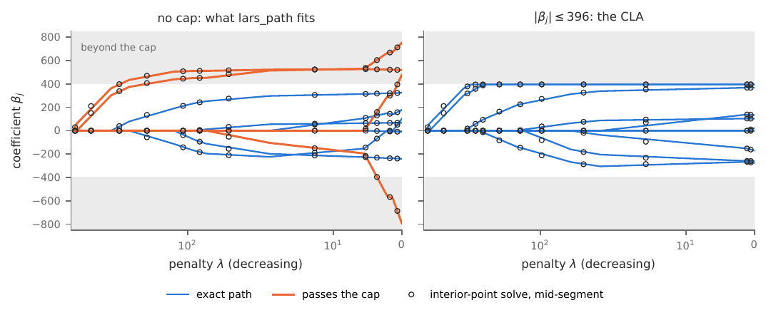
Fig 1: The opening example: the diabetes LASSO path without and with the cap $|\beta_j|\le u=396.1$ . The shaded bands are beyond the cap. Left: the plain LASSO, the path `lars_path` computes; the coefficients that pass the cap are in orange. Right: every coefficient capped. Lines: the exact path, by the CLA in the penalty form. Circles: an interior-point solve at the midpoint of every segment. The horizontal axis is $\lambda$ , decreasing to the right, on a symmetric-log scale: logarithmic above $\lambda_{\max}/50$ and linear below it, so that the end of the path at $\lambda=0$ is shown.

Both panels are exact paths. They come from the Critical Line Algorithm (CLA), which Markowitz (1956) wrote for portfolios, applied to one of the two encodings described below. The open-source package cvxcla (Schmelzer, 2026a) carries them out (Algorithm 1), and the right panel is one call:

from cvxcla import Lasso
knots = Lasso(X, y, lower=-u * np.ones(p), upper=u * np.ones(p)).path

The same call also takes signs (a bound of zero), equality rows a, b and inequality rows g, h, and picks the encoding that fits them.

What this note shows Schmelzer and Hastie (2026) prove that the CLA and the constrained LASSO (Gaines et al., 2018; James et al., 2020) trace the same curve; Table 1 gives the dictionary. Portfolio managers have always needed constraints, such as a budget, position limits and sector exposures, and Markowitz built them into the CLA from the start. So a CLA written for portfolios, with a thin layer that poses the regression as a portfolio, should give exact constrained-LASSO paths. This note shows that it does, or stops with an error where its arithmetic cannot be trusted, and checks every path against references that know nothing of portfolios. The layer is two encodings, Propositions 1 and 2. The propositions need nothing from Schmelzer & Hastie (2026) beyond the classical equivalence of the bound and penalty forms of the LASSO; that paper supplies the general identity of which they are instances. The checks also exposed two defects in the CLA that refused ordinary portfolio problems too, a tie for the largest expected return and a covariance of low rank. Both were fixed in cvxcla 2.6.0 (Schmelzer, 2026a). Drawing the hostile problems of Section 5.4 over more seeds exposed three more, on a design whose columns are nearly collinear: two in the check that a bound held along a segment is still optimal, which refused a correct path, and one in the plain LASSO homotopy, which lost the second of two events at the same $\lambda$ . All three were fixed in 2.7.1, the release used here. Brodie et al. (2009) put an $\ell_1$ penalty on Markowitz portfolios to make them sparse, and a companion note (Schmelzer, 2026b) computes efficient frontiers with a LASSO solver. Both use regression to build portfolios. This note goes the other way. Section 2 recalls the CLA, Section 3 gives the two encodings, Section 4 says where the path starts and ends and collects them in Algorithm 1, Section 5 checks the paths, and Section 6 gives the limits.

Table 1: The dictionary between the two problems (Schmelzer & Hastie, 2026).
regression	portfolio
coefficient $\beta_j$	position in asset $j$
$X^{\top}X$	covariance of the asset returns
$X^{\top}y$	expected returns (penalty form: a benchmark)
$\lVert \beta\rVert _1$	gross exposure
penalty $\lambda$	risk tolerance $\gamma$ (penalty form)
bound $\lVert \beta\rVert _1\le t$	leverage cap $t$ , $\gamma=1/t$ (budget form)
$A\beta=b$ , $l\le\beta\le u$	budget rows and position limits
knot of the LASSO path	turning point of the CLA

The penalty form (Section 3.1) keeps $\lambda$ as the parameter and takes bounds, equality rows $A\beta=b$ and inequality rows $C\beta\le h$ ; it is the general form. The budget form (Section 3.2) keeps the $\ell_1$ budget, as Markowitz’s long-only, fully invested problem with a cash asset, and takes homogeneous constraints such as the zero sum $\mathbf{1}^{\top}\beta=0$ of compositional data in one run.

Related work Exact paths of the constrained LASSO are not new. Gaines, Kim and Zhou (2018) derive a path algorithm from its optimality conditions that takes general linear rows. For $C\beta=0$ alone, the Python package c-lasso (Simpson et al., 2021) has a path algorithm with a small ridge term added. For zero sums on blocks of coefficients, the comlasso algorithm of Jeon et al. (2020) traces the exact path, also with $p>n$ . None was derived with portfolios in mind, so Section 5 runs all three as independent checks. Hobson, Butcher and Lentati (2026) revisit Gaines et al. with CLASSO. The linear system of Gaines et al. is singular whenever a sign constraint binds on a zero coefficient, so CLASSO takes the direction from a small quadratic program instead. In the CLA a sign or a cap is a bound, not a row, so that singularity does not arise. CLASSO adds a ridge when $n<p$ , and its code had not been released when we wrote, so we do not run it. The CLA is an active-set method of the same kind, written for portfolios and used here as released. With $p>n$ the other path algorithms for general constraints add a ridge, which decides where their path ends; the CLA needs none (Section 4). Microbiome studies often have more taxa than samples, so this is the case a user of the zero-sum LASSO meets first. Table 6 collects what each accepts.

Notation The design is $X\in\mathbb{R}^{n\times p}$ , with $n$ observations and $p$ predictors, and the response is $y\in\mathbb{R}^n$ . Write $G=X^{\top}X$ and $c=X^{\top}y$ . The constrained LASSO is $\begin{equation} \label{eq:lasso} \mathrm{L}_\lambda:\quad \min_\beta\ \tfrac12\lVert y-X\beta\rVert _2^2+\lambda\lVert \beta\rVert _1 \quad\text{s.t.}\quad A\beta=b,\quad C\beta\le h,\quad l\le\beta\le u, \end{equation} \qquad(1)$ with $A\in\mathbb{R}^{m\times p}$ , $C\in\mathbb{R}^{k\times p}$ and $l_j\le0\le u_j$ , infinite entries allowed, and a nonempty feasible set. A bound that excludes zero, such as $\beta_j\ge\ell$ with $\ell>0$ , is written as the row $-\beta_j\le-\ell$ . With no rows and infinite bounds it is Tibshirani’s LASSO. We assume, as (Schmelzer & Hastie, 2026) does, that $\mathrm{L}_\lambda$ has a unique minimiser $\beta(\lambda)$ for every $\lambda>0$ . Without constraints this holds when the columns of $X$ are in general position (R. J. Tibshirani, 2013), and with constraints when $X$ has full column rank (Hobson et al., 2026, Theorem 6). For constrained problems with $p>n$ we know of no such result. The checks of Section 5 test optimality, not uniqueness: where the minimiser is not unique, they confirm that the path is a path of minimisers.

2 The Critical Line Algorithm

The CLA starts with the portfolio of highest expected return and lowers the risk tolerance; between corners, the turning points or knots, the optimal portfolio moves along a straight line. Precisely, it solves the family of quadratic programs $\begin{equation} \label{eq:cla} \mathrm{P}_\gamma:\quad \min_x\ \tfrac12\,x^{\top}\Sigma x-(q+\gamma\mu)^{\top}x \quad\text{s.t.}\quad Ax=b,\quad Cx\le h,\quad l\le x\le u, \end{equation} \qquad(2)$ for every $\gamma$ from $+\infty$ down to $0$ , with $\Sigma\succeq0$ . Markowitz’s algorithm (Markowitz, 1956) handles general linear constraints; we write them as equality rows, inequality rows and bounds, the form cvxcla takes. Here $x$ is the vector of holdings, $\Sigma$ the covariance, $\mu$ the expected returns and $\gamma$ the risk tolerance. The term $q$ is a benchmark. With $q=\Sigma\bar x$ the objective is, up to a constant, the tracking variance against a portfolio $\bar x$ less $\gamma\mu^{\top}x$ : the same CLA after the bounds and right-hand side are shifted by $\bar x$ . With $q=0$ it is Markowitz’s problem.

Segments Write $g=\Sigma x-q-\gamma\mu+A^{\top}\nu+C^{\top}\eta$ for the gradient of the Lagrangian. A point $x$ with multipliers $\nu$ and $\eta$ is optimal when $g_j=0$ on the free coordinates $\mathcal{F}=\{j:l_j<x_j<u_j\}$ , $g_j\ge0$ where $x_j=l_j$ , and $g_j\le0$ where $x_j=u_j$ . In addition $\eta\ge0$ , with $\eta_i=0$ on every row that is slack, $C_ix<h_i$ . Call the coordinates at a bound blocked, $\mathcal{B}$ , and the rows held tight active, $\mathcal{R}$ . An active row is held as an equality. In the system below it is stacked under $A$ , with its right-hand side $h_i$ under $b$ and its multiplier $\eta_i$ under $\nu$ ; the slack rows take no part. To keep the display short, $A$ , $b$ and $\nu$ stand for these stacks. With $\mathcal{F}$ , $\mathcal{B}$ and $\mathcal{R}$ fixed, $x_\mathcal{F}$ and $\nu$ solve the bordered system $\begin{equation} \label{eq:border} \begin{bmatrix}\Sigma_{\mathcal{F}\mathcal{F}}&A_\mathcal{F}^{\top}\\A_\mathcal{F}&0\end{bmatrix} \begin{bmatrix}x_\mathcal{F}\\\nu\end{bmatrix} =\begin{bmatrix}q_\mathcal{F}-\Sigma_{\mathcal{F}\mathcal{B}}x_\mathcal{B}\\b-A_\mathcal{B}x_\mathcal{B}\end{bmatrix} +\gamma\begin{bmatrix}\mu_\mathcal{F}\\0\end{bmatrix}, \end{equation} \qquad(3)$ so $x_\mathcal{F}=\alpha+\gamma\delta$ and $\nu=\nu_0+\gamma\nu_1$ are affine in $\gamma$ . The gradient on the blocked coordinates is affine too, $g_\mathcal{B}=g_0+\gamma g_1$ . One factorisation and two right-hand sides give the whole segment.

Events Lowering $\gamma$ , the segment ends at the first of four events (Schmelzer & Hastie, 2026, Section 2.1): a free coordinate reaches a bound, a blocked coordinate’s gradient changes sign, a slack row becomes tight, or an active row’s multiplier falls to zero. Each is the root of an affine function of $\gamma$ , such as $\gamma=-g_{0j}/g_{1j}$ . The coordinate or row concerned changes sides, (3) is solved again, and the walk continues; with no event left, the last segment runs to $\gamma=0$ .

The start As $\gamma\to\infty$ the linear term dominates, and the path starts at a vertex maximising $\mu^{\top}x$ over the feasible set. A linear program finds it. Suppose the maximiser is unique, and as many of its coordinates lie strictly inside their bounds as there are equality rows and rows tight at it. Then the bordered matrix in (3) is nonsingular and the walk can begin. This is the nondegenerate case; cvxcla declines a degenerate start.

3 Two encodings

3.1 The penalty form

The first encoding reads the penalty $\lambda\lVert \beta\rVert _1$ as a cost: every unit of gross position, long or short, costs $\lambda$ units of return. To make that a linear cost, each coefficient is split into a long and a short position, both nonnegative. The constraints on $\beta$ become constraints on the positions, unchanged in kind.

Formally, let $S$ have a column $e_j$ for every $j$ with $u_j>0$ and a column $-e_j$ for every $j$ with $l_j<0$ , so that $\beta=Sz$ with $z\ge0$ . Let $\bar u$ collect the matching bounds $u_j$ and $-l_j$ . A coefficient whose bounds are both zero is fixed and can be dropped. Every $j$ then has at least one column, and $S$ has full row rank.

Proposition 1 (Penalty as cost). For $\lambda>0$ , $\beta(\lambda)=Sz(\lambda)$ , where $z(\lambda)$ solves the CLA instance $\mathrm{P}_\gamma$ with $\Sigma=S^{\top}GS,\quad \mu=-\mathbf{1},\quad q=S^{\top}c,\quad \text{rows } ASz=b,\ CSz\le h,\quad 0\le z\le\bar u,\quad \gamma=\lambda .$ Moreover $q$ lies in the range of $\Sigma$ , so the benchmark reading of Section 2 applies: the program tracks a least-squares fit and pays $\lambda$ for every unit of gross position.

Proof. Up to the constant $\tfrac12\lVert y\rVert ^2$ , the CLA objective at $\gamma=\lambda$ is $\tfrac12\lVert y-XSz\rVert ^2+\lambda\mathbf{1}^{\top}z$ . For a fixed $\beta$ feasible in (1), the smallest $\mathbf{1}^{\top}z$ over $z\ge0$ with $Sz=\beta$ and $z\le\bar u$ is $\lVert \beta\rVert _1$ . The rows hold for every such $z$ , since they constrain only $Sz=\beta$ . It is attained by putting $\beta_j$ on the column of its sign, which respects $\bar u$ because $l_j\le\beta_j\le u_j$ . The minimum of the CLA program over $z$ is therefore the minimum of $\mathrm{L}_\lambda$ over $\beta$ . At a minimiser no coordinate holds both signs, since lowering both by the same amount keeps $\beta$ and reduces the cost by $2\lambda$ times that amount. Hence $Sz(\lambda)$ minimises $\mathrm{L}_\lambda$ , and by uniqueness equals $\beta(\lambda)$ . For the range claim, $c=X^{\top}y$ lies in the range of $G$ , say $c=Gv$ . Since $S$ has full row rank, $v=S\bar x$ for some $\bar x$ , and then $q=S^{\top}GS\bar x=\Sigma\bar x$ , where $S\bar x$ is a least-squares fit. ◻

The covariance $S^{\top}GS$ is singular when both signs of a coefficient are allowed, but (3) is not. For $\lambda>0$ the proof keeps the two halves of a coefficient out of $\mathcal{F}$ together. On the free coordinates $\Sigma$ is then positive definite on the null space of the active rows, the standing assumption of Schmelzer & Hastie (2026, Section 2). The halves come apart only at $\lambda=0$ , which rounding can move to $\gamma\approx10^{-16}$ ; cvxcla treats an event whose parameter is round-off as one at $\gamma=0$ .

Figure 2(a) shows the penalty form on the diabetes data (Efron et al., 2004), where there are no constraints and LARS can check every knot.

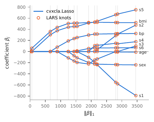
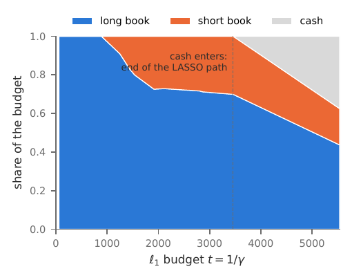
Fig 2: The diabetes LASSO path (Efron et al., 2004), both ways. *(a)* The CLA in the penalty form (lines) and the knots `lars_path` returns (Pedregosa et al., 2011) (circles); all 13 agree to $6.9\times 10^{-14}$ , relative. *(b)* The same path seen by the budget form as a portfolio: the long and short positions $Sw$ and the cash weight $w_0$ share a budget of one, against the leverage $t=1/\gamma$ . Cash enters at $t=\lVert \beta(0)\rVert _1=3460$ , the end of the LASSO path; to its right the least-squares fit is diluted by cash.

3.2 The budget form

With $A\beta=0$ the penalty form starts degenerate (Section 4). The second encoding starts instead from the bound $\lVert \beta\rVert _1\le t$ , a cap $t$ on the leverage, whose path is that of $\mathrm{L}_\lambda$ indexed by $t=\lVert \beta(\lambda)\rVert _1$ (Schmelzer & Hastie, 2026, Theorem 1), and divides by $t$ . The split coefficients then add up to at most one, which is Markowitz’s own setting. A cash asset with no risk and no return holds the rest.

Proposition 2 (Budget as simplex). Suppose $b=0$ and $l_j,u_j\in\{0,\pm\infty\}$ , so that every constraint is homogeneous. Write $\beta=tSw$ with $w\ge0$ , and add a riskless asset $w_0\ge0$ with $\mathbf{1}^{\top}w+w_0=1$ . Then for $t>0$ the bound-form LASSO is the CLA instance $\Sigma=\begin{bmatrix}S^{\top}GS&0\\0&0\end{bmatrix},\quad \mu=\begin{bmatrix}S^{\top}c\\0\end{bmatrix},\quad q=0,\quad \gamma=1/t,$ with rows $\mathbf{1}^{\top}w+w_0=1$ and $ASw=0$ and bounds $w,w_0\ge0$ . This is Markowitz’s long-only, fully invested problem with a cash asset of zero variance and zero return. If $\eta$ is the multiplier of the budget row and $\nu$ those of $ASw=0$ , then $\lambda=t\eta$ and the LASSO’s multipliers for $A\beta=0$ are $t\nu$ .

Proof. As in Proposition 1, $\lVert \beta\rVert _1\le t$ is $\mathbf{1}^{\top}z\le t$ for the split $z=tw$ , and $w_0$ is its slack. The constraint $ASz=0$ is unchanged by the scale $t$ , which is where homogeneity is needed. A nonzero right-hand side would become $b/t=\gamma b$ , a constraint that moves with the parameter. Substituting $z=tw$ gives the objective $t^2(\tfrac12w^{\top}S^{\top}GSw-\gamma c^{\top}Sw)$ plus a constant, and dividing by $t^2>0$ gives $\mathrm{P}_\gamma$ . For the multipliers, multiply the CLA’s stationarity row for a free coordinate, $(S^{\top}GSw)_j-\gamma(S^{\top}c)_j+\eta+(S^{\top}A^{\top}\nu)_j=0$ , by $t$ . This gives $(S^{\top}(G\beta-c))_j+t\eta+(S^{\top}A^{\top}t\nu)_j=0$ , the LASSO’s stationarity condition with penalty $t\eta$ and constraint multipliers $t\nu$ . The cash row reads $\eta\ge0$ while cash is held at zero. ◻

The two forms give the same knots unless the support’s sign vector lies in the span of the active constraint normals (Schmelzer & Hastie, 2026, Corollary 1 and Proposition 1). Under a zero sum that never happens: a nonzero $\beta$ that sums to zero has coefficients of both signs.

4 Where the path starts and ends

The two encodings differ most at the ends of the path. A nondegenerate start lets the walk begin at once; a degenerate one needs a relaxation.

Nondegenerate starts In the penalty form without equality rows the starting vertex is $z=0$ : all positions are closed, because each costs more than it can earn. The first event is the first entry, at $\gamma=\max_j|c_j|$ over the allowed signs, which is LARS’s $\lambda_{\max}$ . Rows $C\beta\le h$ with $h>0$ are slack at $z=0$ , so they leave the start unchanged, and a row joins the active set when the path reaches it, like a bound. With equality rows, or a row with $h_r<0$ that leaves $z=0$ infeasible, the start is the linear program $\min\mathbf{1}^{\top}z$ over $ASz=b$ , $CSz\le h$ , $0\le z\le\bar u$ : the point of smallest $\ell_1$ norm on the constraint set. For generic $A$ and $b\ne0$ it is a unique vertex with $m$ nonzeros, and the path holds still there, $\delta=0$ , until a second coefficient enters. In general, every constrained LASSO path is constant from some $\lambda_0$ on, at a least-squares fit over the feasible points of smallest $\ell_1$ norm, and $\lambda_0$ takes the place of $\lambda_{\max}$ (Schmelzer & Hastie, 2026, Proposition 3). That fit can take a quadratic program to find. Under the fully invested constraint $\mathbf{1}^{\top}\beta=1$ of sparse portfolio regression (Brodie et al., 2009) every long-only $\beta$ in the simplex has $\lVert \beta\rVert _1=1$ , so the starting linear program is not unique; cvxcla starts on the tied face where its quadratic term is smallest, which is that fit.

In the budget form the start, at $\gamma=\infty$ and $t=0$ , is the linear program $\max c^{\top}Sw$ over the simplex: put the whole budget on the best asset. Without equality rows that is the predictor most correlated with the response. It enters with the sign of its correlation and with $\lambda=\lim\eta/\gamma=\max_j|c_j|$ , just as in LARS. Under $\mathbf{1}^{\top}\beta=0$ it is one long and one short position of weight $\tfrac12$ each, the most and the least correlated predictors, entering together. That is why two coefficients leave zero at once in Figure 3. Both starts are generically unique and nondegenerate.

Degenerate starts With $b=0$ the penalty form’s starting vertex is $z=0$ , with no free coordinates for $m>0$ rows. This is a degenerate vertex: the multipliers at the start are not determined by the active set, and (3) is singular. For homogeneous equality rows with signs the budget form is the remedy, because rescaling to the simplex moves the start off the origin. It cannot take rows or caps, which move with the parameter once rescaled (Proposition 2). Caps or inequality rows under a zero sum therefore leave only the penalty form, which starts degenerate there. So do homogeneous rows ( $h=0$ ), such as the ordering constraints of a monotone fit: all are tight at $\beta=0$ .

cvxcla resolves both by relaxation, an implementation device rather than part of the method. It traces the problem twice, with the homogeneous rows relaxed to $h_r=\varepsilon$ and $2\varepsilon$ and a zero sum to $A\beta=\varepsilon Ad$ and $2\varepsilon Ad$ for a generic feasible point $d$ . In release 2.7.1, $\varepsilon$ is $10^{-6}$ times the scale $\lVert c\rVert _\infty/\max_jG_{jj}$ of a coefficient, then $10^{-7}$ and $10^{-8}$ times it if needed. Both runs start nondegenerate. The relaxation enters only the right-hand side of (3), so where the two runs pass through the same active sets their knots are affine in $\varepsilon$ , and $2(\lambda_k,\beta_k)(\varepsilon)-(\lambda_k,\beta_k)(2\varepsilon)$ is the knot at $\varepsilon=0$ . That condition cannot be checked in advance. cvxcla therefore returns the extrapolated path only if a linear program finds multipliers that satisfy the optimality conditions of (1) at every knot and segment midpoint, to $10^{-9}$ relative to $\lVert c\rVert _\infty$ . Otherwise it retries with the next $\varepsilon$ and, after the last, declines. The extrapolation only proposes a path; the certificate is what guarantees the path returned. The paths it returns are checked again, like every other path, in Section 5.

The end of the path As $\lambda\to0^+$ the path ends at the least-squares fit of smallest $\ell_1$ norm under the constraints (Schmelzer & Hastie, 2026, Proposition 3). In the budget form this is where cash leaves its bound, its gradient $\eta$ reaching zero (Figure 2(b)), and the run stops there. With $p>n$ the end is an interpolating fit, and there that event wins a tie, since every correlation vanishes together with $\eta$ . $X^{\top}X$ is then singular, but the bordered system needs a positive definite Hessian only on the null space of the active rows, the standing assumption of Schmelzer & Hastie (2026), so the free set can outgrow the rank of $X$ . The other path algorithms for general constraints add a ridge: $10^{-4}$ in Gaines et al. when $n<p$ , $10^{-3}$ in c-lasso, and $10^{-4}\max_j G_{jj}$ in CLASSO. At that ridge the authors of CLASSO report objectives up to $4\times10^{-2}$ , relative, above the unregularised ones (Hobson et al., 2026, Table 3). Each then traces a nearby problem whose path ends elsewhere.

Algorithm 1: the constrained LASSO path from a CLA.

Form $G=X^{\top}X$ , $c=X^{\top}y$ and the split $S$ of Section 3.1.
If there are equality rows and every constraint is homogeneous ( $b=0$ , $l_j,u_j\in\{0,\pm\infty\}$ , no inequality rows), use the budget form of Proposition 2. Run the CLA from $\gamma=\infty$ and stop when cash leaves zero. A turning point at $\gamma$ with budget multiplier $\eta$ is the knot $\beta=Sw/\gamma$ at $\lambda=\eta/\gamma$ .
Otherwise use the penalty form of Proposition 1 and run the CLA from $\gamma=\infty$ to $0$ . A turning point at $\gamma$ is the knot $\beta=Sz$ at $\lambda=\gamma$ . With $b\ne0$ , or a row with $h_r<0$ , the start is the feasible point of smallest $\ell_1$ norm.
If the start is degenerate, trace the penalty form twice, with the homogeneous rows relaxed by $\varepsilon$ and $2\varepsilon$ , extrapolate the knots to $\varepsilon=0$ , and return the path only if it passes the certificate.
Between two knots $\beta$ is affine in $\lambda$ , so any other point on the path is an interpolation.

cvxcla.Lasso(X, y, a=A, b=b, g=C, h=h, lower=l, upper=u) (release 2.7.1) carries out steps 1–5 and returns the knots. With no constraint at all it traces the plain LASSO by a homotopy instead.

5 Numerical evidence

Each check tests a prediction of Schmelzer & Hastie (2026). Their Lemma 1 makes $\mathrm{L}_\lambda$ and the CLA one parametric quadratic program, so the penalty form should return the knots of $\mathrm{L}_\lambda$ : LARS tests this knot by knot where it applies, and the interior-point solver and the optimality conditions everywhere. Their Theorem 1 and Corollary 1 give the bound form the same knots, so the budget form should return them too: comlasso and c-lasso test this on the zero sums.

5.1 Test problems and checks

Table 2 lists the test problems and their constraints. The diabetes problems use the data of Section 1, with the response centred, and Box is the opening example. Nonnegative carries the one constraint lars_path accepts. In Cholesterol, $h$ is half the least-squares net effect of the three cholesterol measures, and the two rows bind at the end of the path. Pinned fits the first patient exactly, one nonhomogeneous equality row; its path holds still at its starting vertex until $\lambda=4053$ . Wide is a Gaussian design with 8 nonzero coefficients and noise of standard deviation $0.5$ . Zero-sum is a regression on compositional data in the style of Lin et al. (Lin et al., 2014), with the log-shares of $p$ parts as predictors. A composition is known only up to scale, so only a zero sum makes the fit independent of the units. Five parts have nonzero true coefficients. The signs of Zero-sum, signs fall on the even-numbered parts, which the truth meets. The caps of Zero-sum, caps are at half the largest zero-sum least-squares coefficient. Monotone is a Gaussian design with $n=100$ , $p=10$ and an ordered truth, under the rows $\beta_j-\beta_{j+1}\le0$ . Sum to one predicts one unit’s outcomes over 40 periods from those of 20 donors with weights that sum to one. Unlike the classic synthetic control (Abadie et al., 2010), which also requires the weights to be nonnegative, the weights here may be negative; adding the signs would be one more bound. Floor, not in the table, is the diabetes LASSO with $\beta_{\texttt{bmi}}$ at least half its least-squares value, a row that leaves $\beta=0$ infeasible. Its path has 13 knots. It lies within $1.1\times 10^{-10}$ of an interior-point solve at every midpoint and meets the optimality conditions to $1.0\times 10^{-15}$ . sCD14 is the same model on real data from a study of the gut microbiome in HIV infection (Noguera-Julian et al., 2016), as distributed with the R package coda4microbiome (Calle et al., 2023). The predictors come from the counts of 60 bacterial genera in 151 stool samples, and the response is the level of sCD14, a marker of inflammation, in thousands. Each count gets a pseudocount of one, since a zero has no logarithm, and the predictors are the centred log-shares. Its path has 60 knots (Figure 3). Like the diabetes problems, sCD14 is a computational demonstration on real data. No biological inference is intended, and none should be drawn from its path.

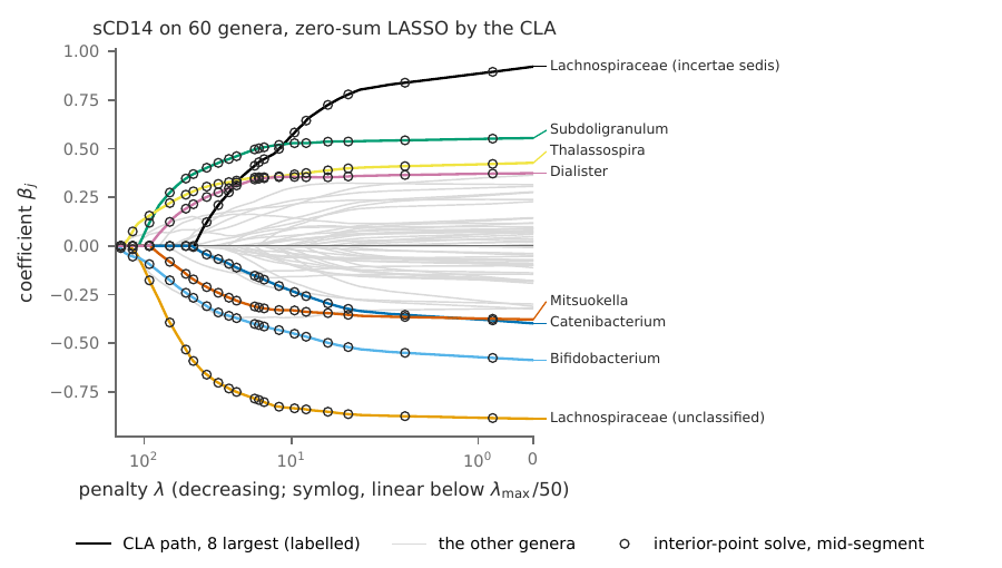
Fig 3: The zero-sum LASSO of sCD14 on the log-shares of 60 genera (Noguera-Julian et al., 2016): the path by the CLA in the budget form. The eight genera largest at $\lambda=0$ are drawn in a colourblind-safe palette (Okabe & Ito, 2008) and labelled at their right-hand end, the others in grey, with an interior-point solve at every third segment midpoint for those eight (circles). Table 2 checks every midpoint of every coefficient. The axis is that of Figure 1: $\lambda$ decreasing, symmetric-log, linear below $\lambda_{\max}/50$ . A computational demonstration; no biological inference is drawn.

Every path comes from cvxcla.Lasso 2.7.1. The bounds are passed even where they are infinite, so that the CLA computes it. Where LARS applies it is the reference, compared knot by knot in both $\lambda$ and $\beta$ . Elsewhere the reference is an interior-point solve (Clarabel through CVXPY, tolerances $10^{-12}$ ) at the midpoint of every segment. There the path is affine in $\lambda$ , so it is known exactly from its two ends. This comparison is only as sharp as the solver. Its largest gap in Table 2 is $4.8\times 10^{-8}$ , relative, on a path whose optimality conditions hold to rounding. The third check evaluates the optimality conditions of (1) directly at every knot and along every segment. Its unknowns are the multipliers $\kappa$ of $A\beta=b$ and $\eta$ of the active rows of $C\beta\le h$ . A linear program chooses them, under $\eta\ge0$ , to minimise one number $\tau$ : the largest violation of all the conditions below, taken jointly. Each condition, written as an inequality $\phi_i(\kappa,\eta)\le0$ that is affine in the multipliers, becomes the row $\phi_i(\kappa,\eta)\le\tau$ , and the program minimises $\tau$ . Its optimum is zero exactly when $\beta$ is optimal. The violation is then evaluated again, exactly, at the multipliers found, so the solver’s own tolerance cannot hide one. A small reported value therefore certifies optimality to that size, and a real violation cannot be masked: no choice of multipliers brings it below the optimum of the program. With $r=G\beta-c+A^{\top}\kappa+C^{\top}\eta$ the conditions are $r_j=-\lambda\operatorname{sign}\beta_j$ on the interior of the support; $|r_j|\le\lambda$ at zero, or only $r_j\ge-\lambda$ under $\beta_j\ge0$ and $r_j\le\lambda$ under $\beta_j\le0$ ; $r_j\le-\lambda$ at a cap $u_j>0$ and $r_j\ge\lambda$ at a floor $l_j<0$ ; $\eta\ge0$ ; and primal feasibility. The check covers each segment whole, not only its midpoint, as Hobson et al. (2026) do. Which coefficients are zero, at a bound or free, and which rows are active, is read off the midpoint. With that fixed, and the multipliers taken affine between the two ends, every condition is affine in $\lambda$ . It holds along the whole segment if it holds at both ends. A linear program finds multipliers at both ends under the midpoint’s pattern, and both ends must fit that pattern: inside a segment no coefficient may change sign or leave a bound, and no row may come loose. A path that is right at both ends of a segment and at its midpoint, but cuts across a knot, fails this check. The published tests include one (test_segment_check_sees_between_samples). With $p=1$ , $y=1$ and the cap $\beta\le\tfrac12$ , the path is zero down to $\lambda=1$ , then $1-\lambda$ up to the cap at $\lambda=\tfrac12$ . A single segment from $(\lambda,\beta)=(\tfrac54,0)$ to $(\tfrac14,\tfrac12)$ misses both knots, yet meets the path at its ends and at its midpoint, where the largest violation of the optimality conditions is 0. The segment check returns 0.25, relative to $\lVert c\rVert _\infty$ . The largest violation, relative to $\lVert c\rVert _\infty$ , is the last column of the table.

Table 2: The CLA against LARS (knot by knot) and against an interior-point solver (IPM, at segment midpoints). *Gap*: largest discrepancy, relative to the largest coefficient. *KKT*: largest violation of the optimality conditions of (1) at every knot and along every segment, relative to $\lVert c\rVert _\infty$ .
problem	constraint	$n$	$p$	knots	ref.	gap	KKT
plain	none	442	10	13	LARS	$6.9\times10^{-14}$	$1.1\times10^{-15}$
nonnegative	$\beta\ge0$	442	10	6	LARS	$2.5\times10^{-15}$	$1.1\times10^{-15}$
wide	none, $p>n$	40	100	53	LARS	$4.2\times10^{-13}$	$6.1\times10^{-16}$
box	$\|\beta_j\|\le u$	442	10	13	IPM	$4.8\times10^{-8}$	$1.2\times10^{-15}$
cholesterol	$\|\beta_{\mathrm{s1}}+\beta_{\mathrm{s2}}+\beta_{\mathrm{s3}}\|\le h$	442	10	14	IPM	$3.4\times10^{-9}$	$1.1\times10^{-15}$
pinned	$x_1^{\top}\beta=y_1$	442	10	18	IPM	$3.6\times10^{-10}$	$1.6\times10^{-15}$
zero-sum	$\mathbf{1}^{\top}\beta=0$	60	30	30	IPM	$1.1\times10^{-10}$	$1.0\times10^{-15}$
zero-sum, signs	$\mathbf{1}^{\top}\beta=0$ , $\beta_{2j}\ge0$	60	30	21	IPM	$2.1\times10^{-11}$	$1.0\times10^{-15}$
zero-sum, caps	$\mathbf{1}^{\top}\beta=0$ , $\|\beta_j\|\le u$	60	30	35	IPM	$1.4\times10^{-9}$	$5.3\times10^{-16}$
monotone	$\beta_j\le\beta_{j+1}$	100	10	13	IPM	$4.6\times10^{-12}$	$9.5\times10^{-16}$
sum to one	$\mathbf{1}^{\top}\beta=1$	40	20	19	IPM	$1.3\times10^{-9}$	$7.5\times10^{-16}$
sCD14	$\mathbf{1}^{\top}\beta=0$	151	60	60	IPM	$8.8\times10^{-10}$	$3.1\times10^{-15}$

5.2 Accuracy

The CLA returns LARS’s knots to $10^{-13}$ , including on the wide design, where 53 knots carry the path to the interpolating fit. The KKT residuals are at the level of rounding throughout, including on the problems LARS cannot take. In positive mode lars_path labels as $\alpha=0$ a point that is the path at $\lambda=30.65$ , so the CLA’s last knot is compared with scipy.optimize.nnls (Lawson & Hanson, 1974) instead.

5.3 Scale and cost

Table 3 extends the test to simulated zero-sum problems of up to $p=500$ parts, each size drawn with three seeds. At that size a midpoint solve per segment would cost more than the path itself, so the table reports only the optimality conditions. They hold to rounding. A second check at the largest size comes from the other encoding. The penalty form, relaxed, returns the same 542 knots to $8.5\times 10^{-15}$ , as it does on every zero-sum problem here (figures/encodings.tex). For a sense of cost, take a grid of 100 interior-point solves (Clarabel through CVXPY, compiled once with $\lambda$ as a parameter). It costs about 90 times as much as the whole CLA path at $p=100$ , 340 times at $p=500$ , and 14 to 110 times on the constrained diabetes and zero-sum problems of Table 2. Each step was run once to warm up and then timed 11 times, 3 times at the sizes of Table 3, on an Apple M4 Pro. The ratios are of the medians; the ratio of any two paired runs stays within 8% of it. These are the only numbers the script does not write into the text. The grid also misses every knot between grid points.

Table 3: The budget form on simulated zero-sum problems of growing size, over three seeds: the range of the knot counts, and the largest KKT violation at every knot and along every segment, as in Table 2.
$n$	$p$	knots	KKT
200	100	100–108	$2.1\times10^{-15}$
400	200	208–224	$3.2\times10^{-15}$
1000	500	538–542	$2.1\times10^{-15}$

5.4 Hostile problems

Table 4 adds problems chosen to make a path algorithm fail, each drawn with ten seeds (7 to 16), and reports the worst case. Correlated is a Gaussian design with $n=100$ and $p=40$ in which every pair of columns has correlation 0.99999. It is run alone, under a box and under a zero sum. Duplicate adds to the diabetes data an eleventh column, bmi plus noise of $1.0\times 10^{-4}$ or $1.0\times 10^{-6}$ times its spread, so that two columns nearly coincide; it is run alone and under the cap of Box. Wide, zero-sum puts a zero sum on Wide, where $p>n$ .

Every path that is traced meets the optimality conditions to $9.6\times 10^{-12}$ or better. The gaps to the references grow with the conditioning. Against LARS the gap stays below $\operatorname{cond}(X)^2$ times the machine epsilon, and LARS’s own KKT residual is at most $2.0\times 10^{-13}$ : both paths are right. The same reading covers a minimiser that is not unique. LARS and the CLA may then trace different paths of minimisers, and a gap between them is no defect as long as both meet the optimality conditions; the certificate, not the agreement, is what each path is held to. Against the interior-point solver the gap reaches $1.5\times 10^{-2}$ on Duplicate, where two nearly identical columns leave the minimiser all but unique: the solver can split the weight between the twins differently at almost the same objective. Even there the solver’s objective is never lower than the path’s by more than $4.8\times 10^{-13}$ , relative, which is within its tolerance.

cvxcla declines Duplicate at $1.0\times 10^{-6}$ without a cap for every seed, because both twins become free (Section 6). Under the cap it declines two of the ten seeds, for the same reason: on those draws both twins become free before the cap binds. On the others they never are both free, and the path is exact. Nothing else is declined. Wide, zero-sum, with $\operatorname{cond}(X)$ near $10^{16}$ , is traced, with the largest residual in the table (Section 4).

Table 4: Hostile problems, through the checks of Table 2, the worst over ten seeds. *Declined*: `cvxcla` stops with an error. The duplicate column is `bmi` plus noise of the given size, relative to its spread.
problem	$n$	$p$	$\operatorname{cond}(X)$	knots	ref.	gap	KKT
correlated	100	40	$5.6\times10^{3}$	43–49	LARS	$1.8\times10^{-9}$	$3.9\times10^{-13}$
correlated, box	100	40	$5.6\times10^{3}$	47–59	IPM	$1.7\times10^{-6}$	$3.0\times10^{-13}$
correlated, zero-sum	100	40	$5.6\times10^{3}$	40–42	IPM	$4.3\times10^{-8}$	$5.1\times10^{-13}$
duplicate $10^{-4}$	442	11	$3.2\times10^{4}$	14–16	LARS	$2.4\times10^{-7}$	$3.2\times10^{-13}$
duplicate $10^{-4}$ , box	442	11	$3.2\times10^{4}$	14–16	IPM	$3.9\times10^{-3}$	$4.0\times10^{-14}$
duplicate $10^{-6}$	442	11	$3.2\times10^{6}$	declined
duplicate $10^{-6}$ , box	442	11	$3.2\times10^{6}$	14 (2 declined)	IPM	$1.5\times10^{-2}$	$1.6\times10^{-15}$
wide, zero-sum	40	100	$5.8\times10^{15}$	50–78	IPM	$2.7\times10^{-8}$	$9.6\times10^{-12}$

5.5 More predictors than observations

A zero sum alone with $p>n$ is covered by comlasso (Jeon et al., 2020) too, so Table 5 puts on Wide ( $n=40$ , $p=100$ , ten seeds) the constraints comlasso does not take. They are nonnegativity; a box at half the largest coefficient of the least-squares fit of smallest norm; two binding inequality rows that cap the net effect of three predictors, as in Cholesterol; the row of Pinned; and a zero sum with the signs of Zero-sum, signs or with the caps of the box. cvxcla declines none of them. Every path meets the optimality conditions to $1.3\times 10^{-9}$ or better along every segment. The largest residuals come at the end of a path, near $\lambda=10^{-4}\lambda_{\max}$ , where the fit almost interpolates; elsewhere they are at rounding. The largest is on one seed of Zero-sum, signs, with $\operatorname{cond}(X)$ near $10^{16}$ . and the interior-point solver agrees to $4.2\times 10^{-6}$ . Its objective is never lower than the path’s by more than $8.1\times 10^{-12}$ , relative. That happens only near the end of a path, where the fit almost interpolates and the objective is small.

Table 5: More predictors than observations, $n=40$ and $p=100$ , under constraints beyond a zero sum, through the checks of Table 2 against the interior-point solver, the worst over ten seeds. None is declined.
Wide with	knots	gap	KKT
nonnegative	48–100	$3.5\times10^{-8}$	$5.6\times10^{-15}$
box	92–315	$2.7\times10^{-6}$	$1.3\times10^{-14}$
inequality rows	50–78	$8.0\times10^{-8}$	$1.4\times10^{-11}$
pinned	51–73	$6.6\times10^{-8}$	$9.7\times10^{-15}$
zero-sum, signs	44–78	$9.3\times10^{-8}$	$1.3\times10^{-9}$
zero-sum, caps	88–389	$4.2\times10^{-6}$	$2.2\times10^{-12}$

5.6 Three independent path algorithms

Three path algorithms derived for the LASSO, with no reference to portfolios, can be run against the CLA. Started at the exact first knot, all three trace its path, up to the ridge two of them add.

comlasso (Jeon et al., 2020) traces the exact path under zero sums on blocks of coefficients, with no ridge and with $p>n$ , so it should agree with the CLA with no workaround. Its authors publish it as an R package built for R 3.2. We load it unchanged (Code availability) and run it on Zero-sum, sCD14 and Wide, zero-sum. It returns the CLA’s knots, to $4.3\times 10^{-15}$ relative to the largest coefficient on the first two and to $1.5\times 10^{-10}$ on Wide, zero-sum over the ten seeds.

The algorithm of Gaines et al. (2018) ships in MATLAB and in Julia. We ported the Julia package to Julia 1 without changing the algorithm (Code availability) and ran it on every problem of Table 2. Started at the exact first knot, where that is simple to state, it agrees with the CLA to $2.9\times 10^{-14}$ on the five such problems with $n\ge p$ : box, cholesterol, plain, sCD14 and zero-sum. On Wide, where $n<p$ , its ridge keeps it $2.8\times 10^{-2}$ away. As shipped, its own start puts it off the path on all 12 problems, by $1.6\times 10^{-5}$ to $1.1\times 10^{2}$ relative to the largest coefficient. It takes the first knot from a linear program that does not involve $y$ , and calls a coefficient active above an absolute threshold of $10^{-4}$ .

c-lasso (Simpson et al., 2021) has a path algorithm for $C\beta=0$ alone, without bounds or signs, so it runs on Zero-sum, sCD14 and Wide, zero-sum. It adds a ridge term $10^{-3}I$ to $X^{\top}X$ , fixed in the package, and that term is the whole of its distance to the CLA. On the first two its 100 grid points lie up to $6.1\times 10^{-5}$ from the CLA path as shipped, relative to the largest coefficient. With the ridge set to $10^{-12}$ by hand they lie $6.0\times 10^{-14}$ from it. With $p>n$ the same ridge is not small. On Wide, zero-sum, c-lasso as shipped lies 0.41 to 0.60 times the largest coefficient from the CLA over the ten seeds, and $1.5\times 10^{-10}$ with the ridge at $10^{-12}$ .

6 Limits and when to use it

When two columns nearly coincide and both become free, moving weight from one to the other barely changes the fit. Unless an active row forbids that move, (3) is then singular to working precision and cvxcla stops (Duplicate at $1.0\times 10^{-6}$ , Table 4). This is the general-position assumption of Section 1, failing in floating point. Dropping or merging one of the two columns before tracing avoids it. A relaxation can also fail its certificate, when knots of the exact path lie closer together than the relaxation moves them; here none was declined. Finally, we do not prove that the walk terminates. The non-terminating examples of Hobson et al. (2026) need multipliers that are not unique, which a nonsingular (3) rules out, and every walk here ended.

When to use it cvxcla.Lasso is for LASSO paths under constraints lars_path does not take: caps, signs on some coefficients, equality and inequality rows and zero sums, also with $p>n$ . It returns the knots at less cost than a grid of interior-point solves (Section 5.3). For the plain or positive LASSO, lars_path is enough. Two nearly identical columns should be merged first. Table 6 lists what each path algorithm accepts.

Table 6: What each exact path algorithm accepts. *Rows*: a bound or sign is written as an inequality row. *All*: `positive=True` makes every coefficient nonnegative, none can be chosen alone. `c-lasso` takes $C\beta=0$ ; comlasso takes zero sums on blocks of coefficients. The ridges are $10^{-3}$ in `c-lasso`, $10^{-4}$ in Gaines et al. when $n<p$ , and $10^{-4}\max_jG_{jj}$ in CLASSO, whose code was not released when we wrote; its column is from its paper (Hobson et al., 2026).
	`lars_path`	`c-lasso`	comlasso	Gaines et al.	CLASSO	`cvxcla`
caps $l\le\beta\le u$	–	–	–	rows	rows	yes
per-coefficient signs	all	–	–	rows	rows	yes
equality rows $A\beta=b$	–	$b=0$	zero sums	yes	yes	yes
inequality rows $C\beta\le h$	–	–	–	yes	yes	yes
zero sums	–	yes	on blocks	yes	yes	yes
$p>n$	yes	yes	yes	yes	yes	yes
$p>n$ without a ridge	yes	–	yes	–	–	yes

We do not compare run times with comlasso, the algorithm of Gaines et al. or c-lasso. None runs here as its authors would run it today: comlasso is R code built for R 3.2 and read under R 4, the algorithm of Gaines et al. is our port of Julia 0.6 code, and c-lasso returns a grid of its own with a ridge. A timing across R, Julia and Python would measure the languages and the ports as much as the algorithms. A user choosing among them should first ask which constraints each accepts, and then time them on their own problem.

7 Conclusion

The checks here support the identity of Schmelzer and Hastie (2026) wherever the encodings reach. On every problem, a CLA written for portfolios returns the exact knots, or stops with an error where its arithmetic cannot be trusted. With $p>n$ the paths stay exact with no ridge, where the other path algorithms for general constraints trace a ridged problem that ends elsewhere.

Data and Code Availability

The software is in preprints/constrained_lasso/ of https://github.com/Jebel-Quant/lasso, under the MIT licence. Each script has a lockfile that fixes Python 3.12 and every package by version and hash. python/make_figures.py computes every path with cvxcla.Lasso 2.7.1 (Schmelzer, 2026a), runs every check, and writes every figure, table and number the text quotes. python/classo_check.py runs c-lasso 1.0.11. R/comlasso_check.R runs comlasso 0.2 under R 4.6.1, locally and in CI. The package was built for R 3.2, and R 4 refuses to install a package built before R 4.0, so the script does not install it. It fetches the package from its authors’ repository at a pinned commit, checks its SHA-256, and reads its functions from the package’s serialized code with lazyLoad, unchanged. comlasso is plain R, with no compiled code, so nothing in it depends on the R 3 build; its one dependency, Rglpk, comes from a dated CRAN snapshot. julia/classopath.jl ports ConstrainedLasso.jl, written for Julia 0.6, to Julia 1.12, with each departure marked; none changes the algorithm. julia/gaines_check.jl runs it in a pinned environment. The sCD14 data are not redistributed: python/fetch_scd14.py downloads coda4microbiome 0.2.4 from CRAN or, should CRAN drop it, from a dated snapshot of Posit Package Manager. It checks the SHA-256 of the tarball, and that of the data file inside it, which is the same byte for byte in both. make figures runs all five, in CI as well.

Every random design is drawn inside python/make_figures.py from a seed recorded there: seed 7 for the problems of Table 2, seeds 7 to 9 for Table 3, and seeds 7 to 16 for Tables 4 and 5. On a fixed platform the discrete results reproduce exactly: the knot counts, which problems are declined, and whether each path passes the certificate. A test runs the problems of Tables 3 and 4 twice and checks that they do. Only residuals near rounding vary, and only in their last digits.

The lockfiles fix the software, not the hardware: those residuals also differ in the last digits on another CPU, so the tests use tolerances between $10^{-12}$ and $10^{-10}$ , and costs are given only as ratios.

Competing interests The author works at Jebel Quant Research, which hosts the code, and maintains cvxcla, which computes every path. The checks are the author’s; the references they compare against are not. LARS, Clarabel, comlasso, ConstrainedLasso.jl and c-lasso were written by others, and the optimality conditions need no solver. There are no other competing interests.

Acknowledgements I thank Trevor Hastie for many helpful discussions.

References

Abadie, A., Diamond, A., & Hainmueller, J. (2010). Synthetic Control Methods for Comparative Case Studies: Estimating the Effect of California’s Tobacco Control Program. Journal of the American Statistical Association, 105(490), 493–505. https://doi.org/10.1198/jasa.2009.ap08746 ↩
Brodie, J., Daubechies, I., De Mol, C., Giannone, D., & Loris, I. (2009). Sparse and stable Markowitz portfolios. Proceedings of the National Academy of Sciences, 106(30), 12267–12272. https://doi.org/10.1073/pnas.0904287106 ↩ 1 2
Calle, M. L., Pujolassos, M., & Susín, A. (2023). coda4microbiome: compositional data analysis for microbiome cross-sectional and longitudinal studies. BMC Bioinformatics, 24, 82. https://doi.org/10.1186/s12859-023-05205-3 ↩
Efron, B., Hastie, T., Johnstone, I., & Tibshirani, R. (2004). Least angle regression. The Annals of Statistics, 32(2), 407–499. https://doi.org/10.1214/009053604000000067 ↩ 1 2 3 4
Gaines, B. R., Kim, J., & Zhou, H. (2018). Algorithms for Fitting the Constrained Lasso. Journal of Computational and Graphical Statistics, 27(4), 861–871. https://doi.org/10.1080/10618600.2018.1473777 ↩ 1 2 3
Hobson, M., Butcher, L., & Lentati, L. (2026). CLASSO: a practical primal path-following algorithm for the constrained LASSO. arXiv. https://doi.org/10.48550/ARXIV.2610.17024 ↩ 1 2 3 4 5 6
James, G. M., Paulson, C., & Rusmevichientong, P. (2020). Penalized and Constrained Optimization: An Application to High-Dimensional Website Advertising. Journal of the American Statistical Association, 115(529), 107–122. https://doi.org/10.1080/01621459.2019.1609970 ↩
Jeon, J.-J., Kim, Y., Won, S., & Choi, H. (2020). Primal path algorithm for compositional data analysis. Computational Statistics & Data Analysis, 148, 106958. https://doi.org/10.1016/j.csda.2020.106958 ↩ 1 2 3
Lawson, C. L., & Hanson, R. J. (1974). Solving Least Squares Problems. Prentice-Hall. ↩
Lin, W., Shi, P., Feng, R., & Li, H. (2014). Variable selection in regression with compositional covariates. Biometrika, 101(4), 785–797. https://doi.org/10.1093/biomet/asu031 ↩
Markowitz, H. M. (1956). The optimization of a quadratic function subject to linear constraints. Naval Research Logistics Quarterly, 3(1–2), 111–133. https://doi.org/10.1002/nav.3800030110 ↩ 1 2
Noguera-Julian, M., Rocafort, M., Guillén, Y., Rivera, J., Casadellà, M., Nowak, P., Hildebrand, F., Zeller, G., Parera, M., Bellido, R., Rodríguez, C., Carrillo, J., Mothe, B., Coll, J., Bravo, I., Estany, C., Herrero, C., Saz, J., Sirera, G., … Paredes, R. (2016). Gut Microbiota Linked to Sexual Preference and HIV Infection. EBioMedicine, 5, 135–146. https://doi.org/10.1016/j.ebiom.2016.01.032 ↩ 1 2
Okabe, M., & Ito, K. (2008). Color universal design (CUD): how to make figures and presentations that are friendly to colorblind people. https://jfly.uni-koeln.de/color/ ↩
Osborne, M. R., Presnell, B., & Turlach, B. A. (2000). A new approach to variable selection in least squares problems. IMA Journal of Numerical Analysis, 20(3), 389–403. https://doi.org/10.1093/imanum/20.3.389 ↩
Pedregosa, F. et al. (2011). Scikit-learn: machine learning in Python. Journal of Machine Learning Research, 12, 2825–2830. ↩ 1 2
Schmelzer, T. (2026b). cvxcla: The Critical Line Algorithm with an Operator Interface in Python. Elsevier BV. https://doi.org/10.2139/ssrn.7583179 ↩ 1 2 3
Schmelzer, T. (2026a). The efficient frontier from a LASSO solver: a numerical check of the CLA–LASSO identity. Journal of Reproducible Statistics, 1. https://doi.org/10.68365/jrepstat.2026.7 ↩
Schmelzer, T., & Hastie, T. (2026). The Critical Line Algorithm and the Constrained LASSO: One Curve, Two Literatures. arXiv. https://doi.org/10.48550/ARXIV.2609.25704 ↩ 1 2 3 4 5 6 7 8 9 10 11 12 13
Simpson, L., Combettes, P. L., & Müller, C. L. (2021). c-lasso – a Python package for constrained sparse and robust regression and classification. Journal of Open Source Software, 6(57), 2844. https://doi.org/10.21105/joss.02844 ↩ 1 2
Tibshirani, R. (1996). Regression Shrinkage and Selection Via the Lasso. Journal of the Royal Statistical Society Series B: Statistical Methodology, 58(1), 267–288. https://doi.org/10.1111/j.2517-6161.1996.tb02080.x ↩
Tibshirani, R. J. (2013). The lasso problem and uniqueness. Electronic Journal of Statistics, 7, 1456–1490. https://doi.org/10.1214/13-EJS815 ↩
Wilson, P. W. F., Meigs, J. B., Sullivan, L., et al. (2007). Prediction of incident diabetes mellitus in middle-aged adults: the Framingham Offspring Study. Archives of Internal Medicine, 167(10), 1068–1074. https://doi.org/10.1001/archinte.167.10.1068 ↩

Cite this article

Schmelzer, T. (2026). The Constrained LASSO is a Portfolio: A numerical check of the CLA–LASSO identity under constraints. Journal of Reproducible Statistics, 1, 10. https://doi.org/10.68365/jrepstat.2026.10

doi: https://doi.org/10.68365/jrepstat.2026.10

Downloads

PDF ePub JATS XML .bib .ris .csl.json Reproducibility package (.zip) da774fd9a0c99c4755bb1ff8c865bae1b4091f5979caff4cc48b25791e2f0e01

https://doi.org/10.68365/jrepstat.2026.10 also supports content negotiation, so reference managers can fetch the citation from the DOI directly. The exports above work without it.