The Efficient Frontier from a LASSO Solver: A numerical check of the CLA–LASSO identity

Thomas Schmelzer

doi:10.68365/jrepstat.2026.7

Research article · Published 2026-10-22 · Open access, CC-BY 4.0

The Efficient Frontier from a LASSO Solver: A numerical check of the CLA–LASSO identity

Thomas Schmelzer¹

¹ Jebel Quant Research, Abu Dhabi · orcid 0009-0009-9771-3501

efficient frontiercritical line algorithmLASSOleast angle regressionportfolio optimisationreproducibility

doi: https://doi.org/10.68365/jrepstat.2026.7 Vol. 1 (2026) · Art. 7 Version 1 how to cite ↓ html pdf (typeset)

✓ Reproduced

Reproducibility record

verified 2026-10-15

Result: Reported results reproduced. All 42 counts and path values reproduce on macOS arm64 and Linux. Residuals near 10⁻¹³ differ in their last digits, as the article states.; ✓ measured
Entry point: cd code/lasso-3e2853642989717c716fed9eca50a3873fa04dd3/preprints/lasso && uv run python/make_figures.py test; ✓ executed
Environment: Python 3.12 from make_figures.py.lock via uv, Linux aarch64 container and macOS arm64, R 4.6.1 with lars 1.3; ✓ measured
Determinism: Seeded.; declared
Archive: the-efficient-frontier-from-a-lasso-solver-a-numerical-check-of-the-cla-lasso-identity-v1-repro.zip · reviewed bundle SHA-256 0b9d144d369821d8ea3ba6d7d4f15aff50c8ff5e0bb0b206c7ef6136f1492983 · https://doi.org/10.5281/zenodo.23554439; ✓ computed
Code: https://github.com/Jebel-Quant/lasso; declared
Data: Open.; declared, route checked

Reproducibility package (.zip, 162 KB) · Zenodo doi:10.5281/zenodo.23554439 · SHA-256 a62bc48c3d0359963c16564bda0a5f9f83e3789a2c53e7f3378824355706e250

$cd code/lasso-3e2853642989717c716fed9eca50a3873fa04dd3/preprints/lasso && uv run python/make_figures.py test

Reproduce: cd code/lasso-3e2853642989717c716fed9eca50a3873fa04dd3/preprints/lasso && uv run python/make_figures.py test · code & data via doi:10.68365/jrepstat.2026.7

Open review

Peer review record

2 rounds · 3 reviewers · signed Full reviewsHide reviews 2026-10-14Minor revision2026-10-15Revised2026-10-15Accepted

The decision letters, the reports the authors read, their answers and the editor's signed decisions, as written. The reports come from the journal's review engine. The authors could have kept this record private until they confirmed the proof.

Round 1Minor revision3 reviewers · response

Minor revisionConfirmed and signed by Matthias Templ2026-10-14 · orcid 0000-0002-8638-5276

Decision letter2026-10-14This note verifies numerically that the mean–variance efficient frontier can be traced with a general LASSO solver (scikit-learn’s lars_path) and no portfolio software, confirming the CLA–LASSO identity of Schmelzer and Hastie to about 10^-13 on simulated factor models, Fama–French portfolios, and 494 S&P 500 stocks, and it contributes a response shift that lets a single positive-LASSO call reach the minimum-variance portfolio. It matters to practitioners and researchers who compute mean–variance frontiers and want corner-exact paths without a dedicated solver. The reviewers found nothing to fix in the writing itself. We would be glad to see the revised version.

Thank you for your submission to JRepStat. We are inviting a minor revision. The reviewers’ points follow, grouped by weight.

This note verifies numerically that the mean–variance efficient frontier can be traced with a general LASSO solver (scikit-learn’s lars_path) and no portfolio software, confirming the CLA–LASSO identity of Schmelzer and Hastie to about 10^-13 on simulated factor models, Fama–French portfolios, and 494 S&P 500 stocks, and it contributes a response shift that lets a single positive-LASSO call reach the minimum-variance portfolio. It matters to practitioners and researchers who compute mean–variance frontiers and want corner-exact paths without a dedicated solver. The reviewers found nothing to fix in the writing itself. We would be glad to see the revised version.

How to read this letter. The decision rests on the items marked required. If a required item seems wrong to you, or cannot be done within this paper, say so in your response letter and give the reason. A reasoned decline is a legitimate answer, and the editor weighs it. Reviewers can be mistaken. Items marked recommended or optional are advice from the reviewers. Adopt them, decline them with a sentence, or leave them for later work. None of that counts against the paper. The reviewer reports below carry the same marks. The editor who signs this decision may weigh an item differently in the accompanying message, and that message prevails.

required (the decision rests on these):

[Reviewer 3] fetch_sp500.py draws the universe from a live Wikipedia page, so a rerun gets a different constituent set. Pin it to a fixed Wikipedia revision (oldid), or state in Section 8 that the stock universe is as-of a date and not exactly reproducible.

recommended:

[visualisation] In Fig 2 (left) and Fig 1(b) the distinction between a plain call and the shifted extension rests on a blue/red contrast. Blue against red is separable for most colour-vision types, but the red region in Fig 2 is described only as “shaded”, so a reader who cannot resolve the hue loses which weights come from the shift. The square markers in Fig 1(b) already add a shape cue; extending that redundancy to Fig 2 (for example a hatch or a boundary line at the stop, labelled) would make both panels legible in greyscale.
[application-and-data] The data-availability statement names the fetch scripts and the pinned snapshots but does not say whether the two snapshot CSVs themselves are archived anywhere citable (for example a Zenodo deposit alongside the GitHub directory). Since the live sources revise, a reader who wants the note’s exact numbers has no way to retrieve the frozen snapshot. Please state where, if anywhere, the two snapshot files can be obtained, or confirm that only the hashes are preserved.
[ethics-and-integrity] Competing interests are not stated explicitly, though the relevant relationships are disclosed in substance: the author’s affiliation (Jebel Quant Research) appears on the title, the paper is a companion to Schmelzer and Hastie [17] co-authored by the author, and the text states that the optimality checks were written by an author of [17] and are therefore not independent. Please add a short competing-interests statement making the commercial affiliation and the authorship link to [17] explicit, so the disclosure is formal rather than inferred.
[methods-soundness] The step ν = ν0 + len(y)*alphas relies on how scikit-learn scales the alphas returned by lars_path relative to the penalised objective. The KKT residuals confirm the scaling empirically, but one sentence stating the convention (why the number of rows is the correct multiplier, and that it is len(y) for both the Cholesky and centred-returns constructions) would let a reader reproduce the mapping without inspecting the solver internals.
[Reviewer 1] state in the abstract and Section 8 that the real-data frontiers are a verification of the method at scale, not investable frontiers. The S&P 500 set is built from current Wikipedia constituents (survivorship) and Yahoo adjusted prices, so a reader should not read a historical or realistic frontier into it.
[Reviewer 1] make the speed claim’s dependence on QP grid resolution explicit. The “tens of times” figure is relative to a 100-point grid, so report the timing ratios in a small table and say how the advantage scales with grid density.
[Reviewer 1] reconcile the two date ranges for the stock data: the body says “July 2021 to May 2026” while the availability section says prices “2021-06-01 to 2026-06-01”.
[Reviewer 2] Fold an explicit check that the recovered ν reaches below the analytically computed νlast into Algorithm 1, so a user without ground truth can confirm every corner was captured.
[Reviewer 2] Give the one-line reason accuracy degrades as |ν0| grows (conditioning of the shifted response) and report the working δ window for each data set, so the default δ=1 is justified rather than asserted.
[Reviewer 2] State the sensitivity of the minimum-variance support to the hard NNLS threshold (1e-9), or justify it, since the support feeds the closed-form minimum-variance end.
[Reviewer 2] Name the 100-point grid as a chosen comparison density and frame the path’s advantage as returning corners exactly at any density, separating that from the raw speed ratio.
[Reviewer 3] Separate single-machine determinism (fixed seeds, bit-identical) from cross-machine last-digit variation in the availability section, and name which in-text numbers the test target asserts and at what tolerance.
[Reviewer 3] Mark the printed code as excerpts and note version preconditions (for example numpy >= 2 for cholesky(upper=True)) so a reader who copies them is not tripped.
[Reviewer 3] Deposit the derived return matrices as a frozen fixture where source licenses allow, or note the fetch scripts’ dependence on the Yahoo API and the monthly CRSP vintage, so the external-data checks stay runnable after those change.

optional:

[visualisation] Fig 1(b) begins its y-axis at 0.5 rather than 0. For a frontier this is a defensible zoom to show curvature, and the inset handles the low-risk end, but a one-line note in the caption that the axis is truncated would prevent the arc’s steepness being read as larger than it is.
[methods-soundness] The identity and its numerical support rest on Σ≻0 with T>n in every tested case; the singular and high-dimensional regimes are set aside explicitly (Section 9, and [17, §7]). A later study could probe behaviour as Σ approaches singularity, but this is outside the present note.
[Reviewer 1] a comparison against a constrained-lasso path algorithm on a two-constraint case (dollar-neutral or 130/30) would show how far the single-call approach generalises.
[Reviewer 2] Report whether tied knots (two assets entering at one step) arose on the real data, and how LARS handled them.
[Reviewer 3] Guard the first branch of the nu_last min() against an empty b>0 slice with an initial, as the second branch already does.

Reviews

Report Reviewer 1recommends acceptThis is a companion numerical note to the theory paper [17], and it does what it sets out to do. It computes the efficient frontier in three settings (long–short under a gross cap, fixed leverage with varying risk appetite, and long-only fully invested) using only a stock LASSO solver, and it checks each returned portfolio two ways: against its own KKT conditions and against an independent quadratic-programming solver. The agreements reported, residuals near 10^-13 to 10^-15 and weight gaps at the same scale, are consistent across the test problem, the factor models of Table 1, the Fama–French portfolios, and the S&P 500 stocks. The reasoning for the one real disagreement, at n=500, where the smaller KKT residual of the path is taken to locate the error in the QP baseline, is sound because KKT is the actual optimality condition rather than a second opinion.

Written by the journal's review engine in the role of the application reviewer, and read by the editor before the decision. How the engine works is on the peer review page.

This is a companion numerical note to the theory paper [17], and it does what it sets out to do. It computes the efficient frontier in three settings (long–short under a gross cap, fixed leverage with varying risk appetite, and long-only fully invested) using only a stock LASSO solver, and it checks each returned portfolio two ways: against its own KKT conditions and against an independent quadratic-programming solver. The agreements reported, residuals near 10^-13 to 10^-15 and weight gaps at the same scale, are consistent across the test problem, the factor models of Table 1, the Fama–French portfolios, and the S&P 500 stocks. The reasoning for the one real disagreement, at n=500, where the smaller KKT residual of the path is taken to locate the error in the QP baseline, is sound because KKT is the actual optimality condition rather than a second opinion.

From an application standpoint the problem is real and the framing is honest. The claim that corner portfolios can be obtained without portfolio software is genuinely useful for the two cases scikit-learn can express, and the response shift of equation (4) and Algorithm 1 are a real practical addition: reaching the minimum-variance portfolio in a single positive-LASSO call, with a ν0 computed in advance, is the kind of detail that saves an implementer real effort. The economic reading of ν as Black’s zero-beta rate, and of the bracketing columns as an interpolation for the maximum-Sharpe portfolio at any rate, is correct and adds value beyond a bare numerical check. Section 9 is candid about the boundaries: a singular covariance, and any mandate needing more than one linear constraint, falls outside what this tool does. Most real mandates do carry more than one constraint, so the practical niche is narrow, and the paper says so clearly, which is the right treatment.

Two points on the data would help a reader. The S&P 500 set is built from current index membership and Yahoo adjusted prices, so it carries survivorship and vintage effects. None of this touches the paper’s claim, which is about numerical agreement of a computation and not about the realism or performance of any frontier, but an applied-finance reader meeting “efficient frontier of 494 S&P 500 stocks” can infer an investable object that is not intended. One or two sentences placing the real data as a scale-and-accuracy check settle it, in the same spirit as the “for illustration only” note on the test problem. Separately, the body and the availability section give different date windows for the stock data, and reconciling them removes a stumble for anyone cross-checking the fetch script.

The speed argument needs one qualification. The accuracy argument is airtight: a path returns the corners exactly where any grid misses them. The speed argument, “a 100-point grid of QPs costs tens of times as much as the path”, depends on the grid resolution, which is a modelling choice. Reporting the ratios in a small table and stating how the margin moves with grid density would let a reader map the claim onto their own setup. The warm-started OSQP comparison is a good addition and already strengthens this part.

On reproducibility the declared package is strong for an applied note: a single self-describing script, a lockfile pinning Python and every dependency to version and hash, published fetch scripts, data snapshots identified by SHA-256, an R cross-check, and a tolerance story that accounts for BLAS-level variation across machines. I did not run it, so I report what is documented rather than a reproduction I performed. The authors also state that the checks were written by an author of [17], which the independent baseline solvers mitigate.

Numbered suggestions to the authors:

recommended Add one or two sentences in the abstract and Section 8 stating that the real-data frontiers verify the method at scale and are not investable frontiers, and noting that the S&P 500 set uses current index membership (survivorship) and adjusted prices.
recommended Report the path-versus-grid timing ratios in a small table and state how the speed advantage depends on the QP grid resolution, so the “tens of times” claim is tied to its grid.
recommended Reconcile the stock-data date windows between the body (“July 2021 to May 2026”) and the availability section (“2021-06-01 to 2026-06-01”).
optional Compare against a constrained-lasso path algorithm on a two-constraint case such as dollar-neutral or 130/30, to show how far the single-call approach extends beyond scikit-learn’s single constraint.

Report Reviewer 2recommends acceptThis note does one job and does it carefully: it checks, numerically and against independent solvers, that the constrained-LASSO path and the Markowitz frontier are the same curve, and it packages a usable recipe for the long-only case. The change of variables in equation (1) is correct and cleanly stated. With X equal to the upper Cholesky factor, X⊤X = Σ and X⊤y = µ, and the identity 1/2 w⊤Σw − µ⊤w = 1/2‖y − Xw‖² − 1/2‖y‖² follows directly, so the mean-variance problem under an ℓ1 cap is the LASSO in constrained form. I checked the signs through to the budget multiplier ν = (µ − Σv)_j on the support, and the parametrisations in Sections 5, 6 and 7 are mutually consistent.

Written by the journal's review engine in the role of the methodology reviewer, and read by the editor before the decision. How the engine works is on the peer review page.

This note does one job and does it carefully: it checks, numerically and against independent solvers, that the constrained-LASSO path and the Markowitz frontier are the same curve, and it packages a usable recipe for the long-only case. The change of variables in equation (1) is correct and cleanly stated. With X equal to the upper Cholesky factor, X⊤X = Σ and X⊤y = µ, and the identity 1/2 w⊤Σw − µ⊤w = 1/2‖y − Xw‖² − 1/2‖y‖² follows directly, so the mean-variance problem under an ℓ1 cap is the LASSO in constrained form. I checked the signs through to the budget multiplier ν = (µ − Σv)_j on the support, and the parametrisations in Sections 5, 6 and 7 are mutually consistent.

The one genuinely new mechanical contribution is the shift in equation (4). Completing the square moves the penalty into the response because X⊤d = 1 makes ν1⊤v equal to νd⊤Xv, so running the nonnegative LASSO on y − ν0 d with penalty ν′ realises the effective multiplier ν0 + ν′ and reaches the segment below where a plain penalised solver stops. This is the right way to recover the part of the frontier that a LASSO solver cannot reach, since it will not take a negative penalty. The detail that scikit-learn reports its alpha divided by the sample count, handled by nu = nu0 + len(y) * alphas, is a place where such notes usually go wrong, and it is right here for both the square X⊤X = Σ construction and the tall centred-returns construction.

The evidence is the kind a methodology reader wants. Each returned portfolio is tested against its own KKT conditions, and separately against baselines that do not share code with the path (Clarabel through cvxpy, quadprog, OSQP). The residuals sit at 1e-13 to 1e-15, and where the path and a baseline disagree the residual identifies the baseline as the less accurate party, which is the correct reading for an interior-point method at a corner. The disclosure that the self-consistency checks were written by an author of the companion paper, with the independence resting on the external solvers, is the honest framing and I accept it. The reproducibility setup is strong: a pinned lockfile, a test command with stated tolerances, data-fetch scripts with dataset hashes, and timings given as machine-portable ratios with absolute times withheld. That is close to what I would hold up as the target for an applied note of this kind.

My reservations are about the recipe’s reliability in a practitioner’s hands, and they are improvements to a sound method rather than doubts about it. The choice of δ in ν0 = νlast − δ max(|νlast|, ‖µ‖∞) is presented through its observed behaviour: on the stock data δ=1e-4 drops the last corner and δ=100 inflates the residual to 2e-11, while on the portfolio data even δ=1e-2 drops the last corner and δ=1 recovers all twelve. The default δ=1 therefore sits inside a window whose lower edge is data-dependent, and a user running a new problem has no way to see a lost corner from the output alone. The method already computes νlast analytically, so the fix is cheap: check that the recovered ν descends below νlast and say so in Algorithm 1, and give the one-line conditioning argument behind “accuracy falls roughly in proportion to |ν0|” so the tradeoff is explained and not only observed. In the same spirit the minimum-variance support is read off an NNLS solution with a fixed 1e-9 cutoff, and a word on how sensitive the recovered support is to that cutoff would close the last gap in the closed-form minimum-variance end.

On Section 9, the speed claim rests on a 100-point QP grid, and the honest statement of the path’s advantage is that it returns the corners exactly at any grid density, which is separate from the raw time ratio. Making that separation explicit would stop a reader reading the ratio as the whole case. None of this changes the note’s conclusions. The paper is correct where I can check it analytically, honest about what it verifies and what it assumes from the companion proofs, and reproducible to a degree most submissions are not.

Numbered suggestions to the authors:

recommended Add to Algorithm 1 an explicit check that the recovered ν descends below the analytically computed νlast, so a user without ground truth can confirm every corner was captured, and mention it in the δ discussion of Section 7.
recommended Give the one-line reason the shifted problem loses accuracy as |ν0| grows (conditioning of y − ν0 d), and report the working δ window for each data set, so the default δ=1 is justified rather than asserted.
recommended State how sensitive the minimum-variance support S is to the 1e-9 NNLS threshold, or justify the threshold, since S determines the closed-form minimum-variance end.
recommended In Section 9, name the 100-point grid as a chosen comparison density and state the path’s advantage as returning corners exactly at any density, kept separate from the speed ratio.
optional Report whether tied knots (two assets entering at one LARS step) occurred on the 99-, 494- or 500-asset problems, and how they were handled, since degeneracy is where a path method is most fragile.

Report Reviewer 3recommends minorI read this as a software-and-reproducibility reviewer: can I run it, is the code sound, and are the reported numbers the code’s numbers? On the first two the answer is largely yes, and the packaging is better than most submissions of this kind. A single Python script that declares its own pinned dependencies, a lockfile that fixes Python 3.12 and every package to an exact version and hash, one documented command to regenerate the figures and numbers and another to run the checks, an R cross-check, and SHA-256 fingerprints for the two external snapshots. The core claim, that the CLA frontier and the LASSO path coincide, rests on simulated data generated inside the script from fixed seeds, so the central verification needs no network and no copyrighted data. That is the right architecture: the load-bearing evidence is self-contained, and the external datasets are scale tests layered on top.

Written by the journal's review engine in the role of the software reviewer, and read by the editor before the decision. How the engine works is on the peer review page.

I read this as a software-and-reproducibility reviewer: can I run it, is the code sound, and are the reported numbers the code’s numbers? On the first two the answer is largely yes, and the packaging is better than most submissions of this kind. A single Python script that declares its own pinned dependencies, a lockfile that fixes Python 3.12 and every package to an exact version and hash, one documented command to regenerate the figures and numbers and another to run the checks, an R cross-check, and SHA-256 fingerprints for the two external snapshots. The core claim, that the CLA frontier and the LASSO path coincide, rests on simulated data generated inside the script from fixed seeds, so the central verification needs no network and no copyrighted data. That is the right architecture: the load-bearing evidence is self-contained, and the external datasets are scale tests layered on top.

I checked the printed code against the APIs it calls. The Cholesky, lstsq, lars_path, lars_path_gram, nnls and interpolation snippets are consistent with current scikit-learn, scipy and numpy, and the alpha-to-ν rescaling (nu = nu0 + len(y) * alphas) and the max_iter guard match the text. I found no demonstrable bug in the printed lines. One version precondition is worth surfacing for readers who copy the snippets: cholesky(Sigma, upper=True) needs numpy 2.0 or later, and lstsq will warn about rcond on some versions. The lockfile presumably pins a compatible numpy, so this is about the excerpts in the paper, not the script.

My one required point concerns the stock-data reproduction. fetch_sp500.py takes the constituent list from a live Wikipedia page and the prices from Yahoo, and the raw data is not redistributable. The paper already documents that a later download differs and sets a 10^-8 tolerance for the baseline drift, which is the responsible thing to do. The remaining gap is the universe itself: a live page means a rerun does not even start from the same set of names, so the “anyone can repeat them” claim of the abstract is only partly met for Section 8. Pinning the fetch to a Wikipedia revision id is a few hours and fixes the universe. If that is impractical, one sentence in Section 8 stating the universe is as-of a date and not exactly reproducible closes the same gap. Either settles it, and neither touches the core result.

The remaining points strengthen the reproducibility story without changing any claim. The availability section mixes two different guarantees: seeds fixed means a single machine should reproduce bit-for-bit, while cross-machine BLAS differences move the last digits, which is why the tolerances exist. Stating those two separately, and naming which in-text numbers (the 7.765, the 2.120, the residual figures, the corner counts) the test target actually asserts, would let a reader see the scope of “regenerates every figure and number” rather than take it on trust. Depositing the derived return matrices as a frozen fixture where the French and Yahoo terms allow would also keep the external checks runnable after the Yahoo API or the monthly CRSP vintage moves, since a fetch script that depends on a third-party API tends to stop running within a year or two. The nu_last computation guards its second branch with an initial but not its first, which would raise on an empty b>0 slice; in practice the minimum-variance support gives a non-empty positive b, so this is a defensive tidy-up only.

The disclosure that the checks were written by an author of [17] is handled correctly, with independent baseline solvers (Clarabel, quadprog, OSQP) carrying the comparison and the scripts published for rerun. That is the right way to manage it.

Numbered suggestions to the authors:

required Pin fetch_sp500.py to a fixed Wikipedia revision (oldid) so the S&P 500 universe is reproducible, or add one sentence in Section 8 stating the universe is as-of a date and not exactly reproducible.
recommended In the availability section, separate single-machine bit-identical determinism (fixed seeds) from cross-machine last-digit variation, and list which in-text numbers make_figures.py test asserts and at what tolerance.
recommended Mark the in-text code as excerpts and state version preconditions, for example that cholesky(Sigma, upper=True) needs numpy 2.0 or later.
recommended Deposit the derived return matrices as a frozen fixture where the source licenses permit, or note in the availability section that the fetch scripts depend on the Yahoo API and the monthly CRSP vintage and may cease to run.
optional Add an initial to the first branch of the nu_last min() to match the second branch and avoid a raise on an empty b>0 slice.

Revision

Authors' response2026-10-15This revision was answered under the earlier rule: a short note on what changed, and a reason for each required point the authors declined.

This revision was answered under the earlier rule: a short note on what changed, and a reason for each required point the authors declined.

The authors' response letter (PDF)

Round 2Accepted3 reviewers

AcceptedSigned by Matthias Templ2026-10-15 · orcid 0000-0002-8638-5276

The editor's note

Final acceptance of version 2, after the editor read the preview of the article.

Decision letter2026-10-15Congratulations, your manuscript has been accepted for publication in JRepStat. Production begins now.

Congratulations, your manuscript has been accepted for publication in JRepStat. Production begins now.

Where it is not on file yet, we still need the following for production.

a valid ORCID iD for every author
a captured computational environment (dependencies/lockfile/container)
a signed determinism attestation for the entry-point command

Reviews

Report Reviewer 1recommends acceptOf the three recommended points and one optional one I raised, the three recommended points are met and the optional one is parked, which is the right call for this note.

Written by the journal's review engine in the role of the application reviewer, and read by the editor before the decision. How the engine works is on the peer review page.

Of the three recommended points and one optional one I raised, the three recommended points are met and the optional one is parked, which is the right call for this note.

Replacing the S&P 500 download with a seeded five-factor simulation settles two of my asks at once. The survivorship and vintage caveat is no longer needed, because there is no real-equity frontier for a reader to mistake for an investable object, and the conflicting date windows disappear with the download. For this journal the change is a net gain: every number in Section 8 except the Fama–French block now regenerates from a seed, and the removed fetch script, lockfile entry and download tolerances simplify the reproducibility story rather than weakening it. Withdrawing the two-machine timing claim and the OSQP 1e-5 remark is consistent with keeping only what the single measured run supports.

My second point, on the speed claim, is substantially addressed. Both Section 8 and Section 9 now name the grid as 100 points, so the “about sixty times” figure is tied to a stated resolution (one to two path solves against roughly a hundred QP solves is internally consistent). The contrast between the 99-portfolio case, where a grid costs about as much as the path, and the 500-stock case, where it costs about sixty times as much, shows how the margin moves with problem size. This covers the practical substance of what I asked for. A small table sweeping grid density was the lighter form of the ask and is not needed for the claim to stand.

The competing-interests statement is clear about the cvxcla maintenance and about where the note uses it, and the method’s independence from that package (scikit-learn or R alone) is correct as stated. Nothing in the revised version raises a new material concern from an application standpoint. The paper is a numerical verification note, the simulated data serve that purpose fully, and the niche (one linear constraint beyond the signs) is stated plainly in Section 9.

Numbered suggestions to the authors: (none — the recommended points are met and the paper is ready as it stands)

Report Reviewer 2recommends acceptI recommended accept last round, and the revision does not disturb that. Of the four recommended points and one optional one I raised, the Section 9 separation of accuracy from speed is now done cleanly (the path finds corners exactly at any density, a grid of QPs misses them, and the speed advantage is stated only where it holds, at scale), and the δ windows are now reported for every data set. The move to a seeded simulated universe in Section 8 removes the last irreproducible download and the competing-interests statement is present and specific; both strengthen the note against the journal’s aims.

Written by the journal's review engine in the role of the methodology reviewer, and read by the editor before the decision. How the engine works is on the peer review page.

I recommended accept last round, and the revision does not disturb that. Of the four recommended points and one optional one I raised, the Section 9 separation of accuracy from speed is now done cleanly (the path finds corners exactly at any density, a grid of QPs misses them, and the speed advantage is stated only where it holds, at scale), and the δ windows are now reported for every data set. The move to a seeded simulated universe in Section 8 removes the last irreproducible download and the competing-interests statement is present and specific; both strengthen the note against the journal’s aims.

What remains is the same small set, none of it blocking. Algorithm 1 still does not carry the explicit check that the recovered ν descends below νlast, which was the cheapest way to let a user see a dropped corner from the output alone, and it is the point I would most like closed since the δ discussion shows how easily the last corner is lost (δ=1e-4 on the stock data, δ=1e-2 on the portfolio data). The conditioning argument behind “accuracy falls roughly in proportion to |ν0|” is still stated as an observation, not explained. The sensitivity of the minimum-variance support to the 1e-9 NNLS cutoff is still unaddressed, and the tied-knot question remains unreported. All four are improvements to a method I judge correct where I can check it analytically, and the note stands without any of them.

Numbered suggestions to the authors:

recommended Add to Algorithm 1 the explicit check that the recovered ν descends below νlast, and mention it in the δ discussion of Section 7, so a dropped last corner is visible from the output.
recommended Give the one-line reason the shifted problem loses accuracy as |ν0| grows (conditioning of y − ν0 d), so the reported δ windows read as explained rather than only measured.
recommended State how sensitive the minimum-variance support S is to the 1e-9 NNLS threshold, or justify the threshold, since S determines the closed-form minimum-variance end.
optional Report whether tied knots (two assets entering at one LARS step) occurred on the 99-, 500- or 116-corner problems, and how they were handled.

Report Reviewer 3recommends acceptOf the one required point and four lighter ones I raised, the required point is settled and two of the recommended ones with it.

Written by the journal's review engine in the role of the software reviewer, and read by the editor before the decision. How the engine works is on the peer review page.

Of the one required point and four lighter ones I raised, the required point is settled and two of the recommended ones with it.

The required point was the live Wikipedia universe in fetch_sp500.py, which made the at-scale Section 8 reproduction start from a different constituent set on every rerun. Replacing the S&P 500 download with a seeded five-factor simulation of 500 stocks over 1,250 days removes the external dependency outright, so the at-scale example now reproduces exactly from the committed code. That is a stronger fix than the oldid pin or the as-of sentence I offered as alternatives, and the two claims that rested on the old data (the two-machine cost ratio and the 1e-5 OSQP miss) are correctly withdrawn rather than carried over. The only remaining external data is the Fama-French portfolio set, and the availability section now records the CRSP vintage, the SHA-256, and that a later download can differ where CRSP revises a return. That closes my point 4 for the data that is still fetched.

The determinism point (my point 2) is addressed: the availability section now separates the software lock from hardware variation, states that last digits differ across CPU and BLAS builds, and gives the tolerance band the tests assert (10^-12 to 10^-9). It does not enumerate which individual in-text numbers the test target checks, but the band and the scope statement cover the substance, and this was recommended.

Two items are still open and neither blocks. The in-text snippets are not marked as excerpts and carry no version precondition, so a reader who copies cholesky(Sigma, upper=True) onto numpy 1.x will hit a TypeError; the lockfile protects the script, not the copied lines. The first branch of the nu_last min() still has no initial while the second does, which in practice is harmless because the minimum-variance support gives a non-empty positive b.

The competing-interests statement is now present and names the note’s two uses of cvxcla, which handles the disclosure well.

Numbered suggestions to the authors:

recommended Mark the in-text code as excerpts and state version preconditions, for example that cholesky(Sigma, upper=True) needs numpy 2.0 or later.
optional Add an initial to the first branch of the nu_last min() to match the second branch and avoid a raise on an empty b>0 slice.

Peer review record (PDF) · How open review works

Abstract

Schmelzer and Hastie prove that Markowitz's Critical Line Algorithm and the LASSO path trace the same curve. This companion note checks that result numerically with a stock LASSO solver, lars_path from scikit-learn, and no portfolio software. It covers long–short portfolios under a leverage cap, fixed leverage with varying risk appetite, and the classical long-only, fully invested frontier. Every corner the path returns meets its own optimality conditions to about 10⁻¹³ and agrees with independent quadratic-programming solvers, on factor models of up to 500 assets, on the Fama–French size and book-to-market portfolios, and on five years of simulated daily returns of 500 stocks. A plain call stops the long-only path at the maximum-Sharpe portfolio; shifting the response once, by an amount computed in advance, lets a single call reach the minimum-variance portfolio. The script, its checks, a script that fetches the data, and an R cross-check are published, with a locked environment, so that anyone can repeat them.

Introduction

As the trade-off between expected return and variance changes, the optimal portfolio moves along straight lines and changes direction only at finitely many corner portfolios, where an asset enters or leaves. Markowitz’s Critical Line Algorithm (CLA) (Markowitz, 1956) walks from one corner to the next. The LASSO (Tibshirani, 1996) behaves the same way as its penalty moves, and the LARS algorithm (Efron et al., 2004) walks its corners, which statisticians call knots. Schmelzer and Hastie (2026) prove that after a change of variables the two paths coincide. This note checks that result numerically, by computing frontiers with a LASSO solver and testing them against independent solvers, in three settings:

long–short under a gross-exposure cap, where the plain LASSO path is the frontier (Section 5);
fixed leverage with varying risk appetite, where the same path is rescaled (Section 6);
long only and fully invested, where the nonnegative LASSO path, shifted once, covers the whole frontier in one call (Section 7, Algorithm 1).

The usual alternative is to solve a quadratic program on a grid of tilts. Each solve is only as accurate as its tolerance, and every corner between two grid points is missed. A path algorithm returns the corners themselves, and every other frontier portfolio is a linear interpolation between two of them.

Background

Markowitz (1952) called a portfolio efficient if no other has a higher expected return $E$ without a higher variance $V$ , or a lower $V$ without a lower $E$ . Traced by minimising $\tfrac12V-\lambda E$ over fully invested portfolios for $\lambda\ge0$ , they form the efficient frontier, with the minimum-variance portfolio at $\lambda=0$ . The CLA followed (Markowitz, 1956). Tobin (1958) and Sharpe (1964) moved the picture to the $(\sigma,E)$ plane, where Sharpe located the dominant portfolio, the one with the highest Sharpe ratio, at the tangent from the riskless rate.

The LASSO fits least squares under $\lVert \beta\rVert _1\le t$ and so shrinks and selects at once. Its path is piecewise linear in $t$ . Osborne, Presnell and Turlach (2000) gave a homotopy for it and Efron et al. (2004) gave LARS, which also covers the positive LASSO. Later practice moved to coordinate descent on a grid of penalties (Friedman et al., 2010), which, like a grid of tilts, returns points rather than corners.

The two literatures developed for decades without citing each other (Schmelzer & Hastie, 2026, Section 5). The best-known bridge, Brodie et al. (2009), read a Markowitz problem with a gross-exposure penalty as a LASSO, but swept the penalty at a fixed target return rather than tracing the frontier. Fan, Zhang and Yu (2012) ran LARS along the gross-exposure cap of the minimum-variance portfolio. They removed the budget by regressing on a reference asset, which leaves an $\ell_1$ constraint that is no longer the LASSO’s, so their path is an approximation.

The test problem

The test problem is the seeded 20-asset example of Figure 1 in Schmelzer & Hastie (2026): a five-factor covariance $\Sigma=\operatorname{diag}(d)+U\operatorname{diag}(\delta)U^{\top}$ , and $\mu$ the sample mean of 50 days of returns simulated from it. Its units are arbitrary and its expected returns large against its risk, so Sharpe ratios reach $2.1$ per period, far above anything real assets offer. It is for illustration only; Section 8 adds real portfolio returns and a larger universe on a daily scale. The companion script python/make_figures.py regenerates every figure and number in the note, and its tests check each against a tolerance. The statement on code and data availability at the end says where to find it.

From mean–variance to least squares

Let $\Sigma\succ0$ be the covariance of $n$ assets and $\mu$ their expected returns. With the Cholesky factor $\Sigma=LL^{\top}$ , set $X=L^{\top}$ and $y=L^{-1}\mu$ , so that $X^{\top}X=\Sigma$ and $X^{\top}y=\mu$ . Then for every portfolio $w$ $\begin{equation} \label{eq:square} \tfrac12\,w^{\top}\Sigma w-\mu^{\top}w \;=\; \tfrac12\lVert y-Xw\rVert _2^2-\tfrac12\lVert y\rVert _2^2 , \end{equation} \qquad(1)$ and under any constraints the mean–variance problem is a least-squares problem.

X = np.linalg.cholesky(Sigma, upper=True)  # X.T @ X == Sigma
y = np.linalg.lstsq(X.T, mu)[0]            # X.T @ y == mu
w = np.linalg.lstsq(X, y)[0]               # unconstrained optimum Sigma^{-1} mu

The last line solves the normal equations $X^{\top}Xw=X^{\top}y$ , which are $\Sigma w=\mu$ . With constraints, the optimality conditions become normal equations restricted to the assets held, a linear system in the trade-off parameter. The weights stay linear until the holdings change, and those changes are the corners. The substitution is a change of variables, not a statistical model: $X$ has one row per asset, and $y$ is not data (Schmelzer & Hastie, 2026, Section 4).

Only $X^{\top}X$ and $X^{\top}y$ matter, so any square root of $\Sigma$ will do. If $\Sigma$ is a sample covariance from a $T\times n$ return matrix $R$ with $T>n$ , the centred returns $X=(R-\mathbf 1\bar r^{\top})/\sqrt{T-1}$ work, with $y$ from lstsq. For a factor model, stacking $\operatorname{diag}(d)^{1/2}$ over $\operatorname{diag}(\delta)^{1/2}U^{\top}$ gives an $(n+k)\times n$ matrix with no factorisation at all, and $y=(\operatorname{diag}(d)^{-1/2}\mu,\,0)$ . Both reproduce the Cholesky path to rounding.

Long–short with a leverage cap

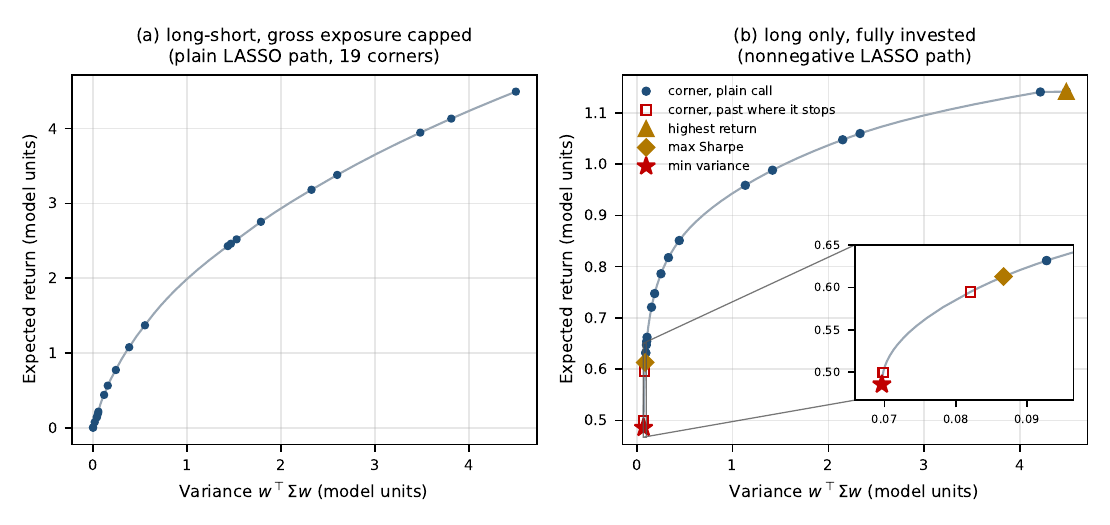
Fig 1: Both frontiers of the test problem, computed with a LASSO solver. *(a)* Long–short under a gross-exposure cap. *(b)* Long-only, fully invested: blue corners come from a plain call, red squares are the two it misses (Section 7). A triangle marks the highest-return portfolio, a diamond the maximum-Sharpe and a star the minimum-variance portfolio; the inset magnifies the low-risk end.

Parameters. $\lambda$ : the tilt, or risk appetite. $c$ : the gross-exposure cap, and $\kappa$ : its multiplier, the LASSO penalty of Sections 5 and 6. $t=\mathbf 1^{\top}v=1/\lambda$ : the budget of the rescaled long-only problem, and $\nu$ : its multiplier, the LASSO penalty of Section 7.

With the gross exposure $\lVert w\rVert _1$ capped at $c$ , $\begin{equation} \label{eq:mark} \min_w\ \tfrac12\,w^{\top}\Sigma w-\mu^{\top}w \qquad\text{s.t.}\qquad \lVert w\rVert _1\le c \end{equation} \qquad(2)$ is, by (1), the LASSO in constrained form, the observation behind the sparse portfolios of Brodie et al. (2009). Its penalised form is $\min_\beta\tfrac12\lVert y-X\beta\rVert _2^2+\kappa\lVert \beta\rVert _1$ , where $\kappa\ge0$ is the multiplier of the cap and $c=\lVert \beta(\kappa)\rVert _1$ . So the LASSO path is the frontier of (2) (Schmelzer & Hastie, 2026, Theorem 1), and scikit-learn (Pedregosa et al., 2011) computes it:

_, _, B = lars_path(X, y, method="lasso")  # columns: start, corners, end
_, _, B = lars_path_gram(Xy=mu, Gram=Sigma, n_samples=len(mu), method="lasso")

The second line gives the same path from $(\Sigma,\mu)$ alone. In R the lars package (Hastie & Efron, 2022) traces it too:

library(lars)
X <- chol(Sigma)                          # t(X) %*% X == Sigma
y <- backsolve(X, mu, transpose = TRUE)   # t(X) %*% y == mu
fit <- lars(X, y, type = "lasso", normalize = FALSE, intercept = FALSE)
B <- t(coef(fit))                         # columns: start, corners, end

It has no positivity constraint, so the long-only path of Section 7 needs scikit-learn. On the test problem the path has 21 columns: the empty portfolio at the start, 19 corners, each adding one asset, and the end. The path starts at $w=0$ , which is optimal while $\kappa\ge\max_j|\mu_j|$ , and ends at $\kappa=0$ , where the cap stops binding at $w^\star=\Sigma^{-1}\mu$ with $\lVert w^\star\rVert _1=7.765$ . That end maximises $\mu^{\top}w-\frac12w^{\top}\Sigma w$ , the second-order approximation to expected log growth, so it is the Kelly portfolio (Kelly, 1956). Since $\Sigma^{-1}\mu$ also maximises the scale-free Sharpe ratio, it points towards the maximum-Sharpe portfolio. On the test problem the Sharpe ratio rises from corner to corner, from $0.539$ at the first to $\sqrt{\mu^{\top}\Sigma^{-1}\mu}=2.120$ at the end, although nothing shown here says it must. Neither end is the minimum-variance portfolio, which needs the budget $\mathbf 1^{\top}w=1$ that (2) lacks.

Fixed leverage, varying risk appetite

A mandate usually fixes the leverage, say $c=2$ , and varies risk appetite through a tilt $\lambda>0$ . Substituting $w=\lambda v$ in $\min\tfrac12w^{\top}\Sigma w-\lambda\mu^{\top}w$ subject to $\lVert w\rVert _1\le c$ gives (2) with cap $c/\lambda$ . The same path therefore serves: a column $\beta$ with $t=\lVert \beta\rVert _1$ , scaled to $w=(c/t)\beta$ , is optimal at tilt $\lambda=c/t$ .

t = np.abs(B[:, 1:]).sum(0)             # gross exposure of each column
W, tilts = B[:, 1:] * (c / t), c / t    # the same portfolios at leverage c

At $c=2$ the columns cover tilts from $745.6$ down to $0.2576$ . Below that the cap is slack and the solution $\lambda\Sigma^{-1}\mu$ shrinks to zero, so the path covers every tilt.

Long only, fully invested

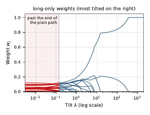
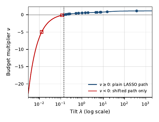
Fig 2: The long-only path of the test problem against the tilt $\lambda$ . *Left:* the weights; blue where a plain call supplies them, red (shaded) where it does not. *Right:* the budget multiplier $\nu=(\mu-\Sigma v)_j$ , $j$ on the support. A plain call covers $\nu\ge0$ and ends at $\nu=0$ , $\lambda=0.1414$ (dashed); the shift (4) reaches the two further corners (squares) where $\nu<0$ .

The classical frontier requires $w\ge0$ and $\mathbf 1^{\top}w=1$ . Substituting $w=\lambda v$ and using (1) turns the tilted problem into $\begin{equation} \label{eq:nnls} \min_v\ \tfrac12\lVert Xv-y\rVert _2^2 \qquad\text{s.t.}\qquad \mathbf 1^{\top}v=t,\ \ v\ge0, \qquad t=1/\lambda , \end{equation} \qquad(3)$ with $w=v/t$ (Schmelzer & Hastie, 2026, Proposition 3). For $v\ge0$ the budget is $\lVert v\rVert _1$ , so (3) is the nonnegative LASSO, whose penalty $\nu$ is the multiplier of the budget. lars_path(…, positive=True) traces it, and each column divided by its sum is a corner portfolio at tilt $1/\mathbf 1^{\top}v$ .

The stop. Called on $(X,y)$ the path runs from $\nu=\max_j\mu_j$ down to $\nu=0$ and stops there, because a LASSO solver takes no negative penalty. (If every $\mu_j\le0$ it returns only the origin.) On the test problem that gives 17 corners, down to tilt $0.1415$ . The stopping point $v_0=\arg\min_{v\ge0}\frac12v^{\top}\Sigma v-\mu^{\top}v$ is the end of Section 5 with long-only weights. Writing $v=sw$ with $\mathbf 1^{\top}w=1$ and maximising over the scale $s\ge0$ first leaves $\frac12(\mu^{\top}w)^2/w^{\top}\Sigma w$ , half the squared Sharpe ratio, so $v_0/\mathbf 1^{\top}v_0$ is the long-only maximum-Sharpe portfolio, at tilt $0.1414$ . The frontier continues beyond it: the budget still binds while $\nu$ turns negative (Figure 2), which a constraint allows and a penalty does not (Schmelzer & Hastie, 2026, Section 3.4). The stop is a property of the penalised form that LASSO solvers use.

The shift. Completing the square once more moves the penalty into the response: $\begin{equation} \label{eq:shift} \tfrac12\lVert Xv-y\rVert _2^2+\nu\,\mathbf 1^{\top}v =\tfrac12\lVert Xv-(y-\nu d)\rVert _2^2+\text{const}, \qquad X^{\top}d=\mathbf 1 . \end{equation} \qquad(4)$ If the nonnegative LASSO runs on $y-\nu_0d$ for some $\nu_0<0$ , its penalty $\nu'\ge0$ acts as $\nu=\nu_0+\nu'$ on the original problem, and one path covers every $\nu\ge\nu_0$ . For the Cholesky factor $d=(X^{\top})^{-1}\mathbf 1$ ; for a tall $X$ least squares returns the minimum-norm solution. lars_path reports $\nu'$ divided by the number of rows, and it stops after 500 steps unless told otherwise, which a large problem needs:

d = np.linalg.lstsq(X.T, np.ones(len(mu)))[0]   # solves X.T @ d == 1
alphas, _, V = lars_path(X, y - nu0 * d, method="lasso", positive=True,
                         max_iter=10 * len(mu))
nu = nu0 + len(y) * alphas                      # budget multiplier per column
corners = V[:, 1:-1]                            # drop the origin and the end
W, tilts = corners / corners.sum(0), 1 / corners.sum(0)

Choosing $\nu_0$ . Any $\nu_0$ below the last corner works, and the last corner is known in advance. Beyond it the portfolio holds the minimum-variance support $S$ , which is the support of $\arg\min_{u\ge0}\lVert Xu-d\rVert _2$ (Lawson & Hanson, 1974). There $v_S=a-\nu b$ with $a=\Sigma_{SS}^{-1}\mu_S$ and $b=\Sigma_{SS}^{-1}\mathbf 1$ , and the segment stays optimal while $\nu<a_i/b_i$ for $b_i>0$ and, for $j\notin S$ with $\Sigma_{jS}b>1$ , while $\nu\le(\mu_j-\Sigma_{jS}a)/(1-\Sigma_{jS}b)$ . The smallest bound is the last corner $\nu_{\mathrm{last}}$ :

S = nnls(X, d)[0] > 1e-9                         # minimum-variance support
a = np.linalg.solve(Sigma[np.ix_(S, S)], mu[S])
b = np.linalg.solve(Sigma[np.ix_(S, S)], np.ones(S.sum()))
h = 1 - Sigma[np.ix_(~S, S)] @ b
g = mu[~S] - Sigma[np.ix_(~S, S)] @ a
nu_last = min((a[b > 0] / b[b > 0]).min(),
              (g[h < 0] / h[h < 0]).min(initial=np.inf))
nu0 = nu_last - max(abs(nu_last), np.abs(mu).max())

A fixed $\nu_0$ would not work, because $\nu_{\mathrm{last}}$ varies widely: it is $-4.95$ on the test problem, $-11.9$ on one of the models of Table 1, $-0.190$ on the stock data and $-0.0118$ on the portfolio data of Section 8, where $\mu$ is small. The margin $\delta$ in $\nu_0=\nu_{\mathrm{last}}-\delta \max(|\nu_{\mathrm{last}}|,\lVert \mu\rVert _\infty)$ has to be large enough that the end of the path does not merge with the last corner, and small enough not to cost accuracy, which falls roughly in proportion to $|\nu_0|$ . On the stock data $\delta=10^{-4}$ loses the last corner; from $\delta=10^{-2}$ to $1$ all 116 are found with KKT residuals below $5\times10^{-13}$ , and at $\delta=100$ the residual has grown to $3\times10^{-11}$ . On the portfolio data even $\delta=10^{-2}$ loses the last corner, and $\delta=1$ finds all 12. The code takes $\delta=1$ . The minimum-variance portfolio itself is the limit $\nu\to-\infty$ ; on the final segment it is $w_S\propto\Sigma_{SS}^{-1}\mathbf 1$ .

What $\nu$ means. By (4) the point with multiplier $\nu$ solves the same problem with $\mu$ replaced by $\mu-\nu\mathbf 1$ , so it is the long-only maximum-Sharpe portfolio at risk-free rate $r=\nu$ , Black’s zero-beta rate (Black, 1972), a classical result. What the LASSO adds is that the rate is the path’s own parameter, so for $\nu_0<r<\max_j\mu_j$ the maximum-Sharpe portfolio is an interpolation between the two columns that bracket $r$ :

assert nu[-1] < r < nu[0]                        # the path covers the rate r
k = np.argmax(nu < r)                            # first column past r
s = (nu[k - 1] - r) / (nu[k - 1] - nu[k])
w_r = V[:, k - 1] + s * (V[:, k] - V[:, k - 1])
w_r /= w_r.sum()                                 # max-Sharpe portfolio at r

Weights versus frontier. Between corners the weights are linear in the tilt $\lambda$ (or, in Section 5, in the cap $c$ ) and the variance is quadratic, so each piece of the frontier is an arc. Traced by the tilt $\lambda$ at fixed constraints (Sections 6 and 7), the frontier has no kinks, since its slope $\mathrm dE/\mathrm dV=1/(2\lambda)$ varies continuously. The corners then show only in the weights (Figure 2). The long–short path of Section 5 is traced by the cap instead and does kink (Figure 1(a)).

Algorithm 1: the long-only frontier from lars_path.

Build $X,y$ with $X^{\top}X=\Sigma$ , $X^{\top}y=\mu$ , or use lars_path_gram with Xy=mu - nu0.
Solve $X^{\top}d=\mathbf 1$ , compute $\nu_{\mathrm{last}}$ and set $\nu_0$ as above.
Run the positive LASSO on $y-\nu_0d$ with max_iter well above $n$ , and recover $\nu=\nu_0+n_{\mathrm{rows}}\alpha$ .
Drop the first and last columns; each remaining $v/\mathbf 1^{\top}v$ is a corner, at tilt $1/\mathbf 1^{\top}v$ .
Take the minimum-variance end as $w_S\propto\Sigma_{SS}^{-1}\mathbf 1$ , and any other point by interpolation, in $1/\lambda$ for a tilt or in $\nu$ for a rate.

Numerical evidence

Two kinds of evidence are reported. The first needs no second solver: each portfolio the path returns is checked against its own optimality conditions. For the cap with multiplier $\kappa$ these are $(\mu-\Sigma w)_j=\kappa\,\mathrm{sign}(w_j)$ on the support and $|(\mu-\Sigma w)_j|\le\kappa$ off it; for the long-only problem at tilt $\lambda$ they are $(\Sigma w-\lambda\mu)_j=\gamma$ on the support and $\ge\gamma$ off it, with $\mathbf 1^{\top}w=1$ and $w\ge0$ . The KKT residual is the worst violation, divided by $\lVert \mu\rVert _\infty$ or by the size of the gradient. The second compares with baselines that are independent of the path. The long–short problems go to Clarabel, an interior-point solver, through cvxpy; the long-only problem goes to quadprog, the active-set method of Goldfarb and Idnani (1983).

Long–short. Every column has a KKT residual below $2.6\times10^{-15}$ , and below $2.9\times10^{-15}$ once rescaled to fixed leverage. At each column’s cap Clarabel matches the path to $3.0\times10^{-7}$ at the corners and $1.4\times10^{-11}$ inside segments. The gap at the corners is the baseline’s, since interior-point methods are least accurate where the holdings change. At fixed leverage the figures are $6.2\times10^{-6}$ and $1.9\times10^{-11}$ .

Long only. The shifted path finds 19 corners on the test problem, the 17 of a plain call and two more at tilts $0.1158$ and $0.0128$ . They match the QP to $6.0\times10^{-13}$ , points inside segments to $7.9\times10^{-14}$ , the minimum-variance end to $1.0\times10^{-16}$ , and the maximum-Sharpe portfolio at $r=0$ to $3.4\times10^{-15}$ . The corners and the minimum-variance end have KKT residuals below $3.6\times10^{-14}$ . Table 1 repeats both checks on other sizes and seeds. Where the two disagree, at $n=500$ , the residual shows that the gap of $6.7\times10^{-11}$ is the QP’s. The number of corners need not equal the number of assets, because some assets leave and re-enter.

Table 1: Algorithm 1 on five-factor models, three seeds each: the worst KKT residual over the corners and the minimum-variance end, the largest $\ell_\infty$ weight discrepancy against an independent active-set QP at the same tilt, and the same discrepancy at the minimum-variance end.
$n$	seeds	corners	$\nu_{\mathrm{last}}$	KKT residual	worst corner	min.-variance end
20	3	19	$-0.57$ to $0.12$	$1.1\times10^{-14}$	$8.6\times10^{-14}$	$2.4\times10^{-16}$
50	3	49	$-11.9$ to $-0.74$	$1.0\times10^{-13}$	$1.5\times10^{-13}$	$1.7\times10^{-16}$
100	3	99–103	$-0.56$ to $-0.38$	$2.5\times10^{-14}$	$1.1\times10^{-11}$	$3.3\times10^{-16}$
500	3	503	$-0.45$ to $-0.26$	$2.1\times10^{-13}$	$6.7\times10^{-11}$	$4.3\times10^{-16}$

Portfolio returns. The daily value-weighted returns of the 100 portfolios that Fama and French form on size and book-to-market (French, n.d.), from January 2016 to December 2025, are free to download from their Data Library, and a script published with the code fetches them. One portfolio misses 250 days and is dropped, which leaves 99 portfolios over 2514 days. With the centred returns as $X$ the last corner sits at $\nu_{\mathrm{last}}=-0.0118$ , eleven times $\max_j|\mu_j|$ below zero. Algorithm 1 returns all 12 corners. They match the QP to $2.1\times10^{-13}$ and have KKT residuals below $3.9\times10^{-14}$ , and the minimum-variance portfolio, which holds 7 of the portfolios, matches to $1.6\times10^{-15}$ . Diversified portfolios are highly correlated, so the frontier turns only 12 times and a grid of QPs is cheap here.

Stock returns. The second data set tests the method at scale. It is simulated, so it needs no download and every rerun reproduces it: daily returns of 500 stocks over 1250 days, about five years, from a five-factor model with a market factor of 1% daily volatility, four style factors of 0.5%, idiosyncratic volatility between 1% and 3%, and expected returns around five basis points a day. Unlike the test problem, $\mu$ and $\Sigma$ are both estimated from the returns. With the centred returns as $X$ the last corner sits at $\nu_{\mathrm{last}}=-0.190$ , about sixty times $\max_j|\mu_j|$ below zero. Algorithm 1 returns all 116 corners in the time of about one QP solve, so a 100-point grid of QPs costs 75 to 95 times as much as the path and still misses the corners. Warm-starting narrows the gap without closing it: OSQP (Stellato et al., 2020), set up once so that its factorisation is reused, with each tilt changing only the linear term and each solve starting from the last, needs a sixth to a third of the cold grid’s time at tolerance $10^{-6}$ and agrees with the cold QP to $3.7\times10^{-12}$ at every grid point. Absolute times depend on the machine and are not reported. Every corner has a KKT residual below $4.7\times10^{-13}$ and matches its QP to $8.6\times10^{-13}$ , and the minimum-variance portfolio, which holds 63 stocks, matches to $5.8\times10^{-16}$ .

When to use it

The path beats a grid of QP solves, cold- or warm-started, on accuracy, since it finds the corners exactly. On speed it wins at scale, on the 500 simulated stocks; on a problem as small as the Fama–French portfolios its lead shrinks to a factor of three or four. LARS is in R and scikit-learn, the positive LASSO only in scikit-learn, so corner portfolios need no portfolio software, and one call shows that the knots of a LASSO path and the turning points of a frontier are the same points. It is the wrong tool when $\Sigma$ is singular, where the identity is not known to survive (Schmelzer & Hastie, 2026, Section 7), or when the portfolio needs more than one linear constraint. The LASSO that scikit-learn solves has exactly one besides the signs, $\lVert \beta\rVert _1\le t$ : the gross-exposure cap of Sections 5 and 6, or, with positive=True, the budget $\mathbf 1^{\top}w=1$ of Section 7. The signs are either all free or all nonnegative. A dollar-neutral book adds the equality $\mathbf 1^{\top}\beta=0$ , and a $130/30$ book needs the budget and the gross cap at once. Path algorithms for a LASSO with general linear constraints exist (Gaines et al., 2018; James et al., 2020), but not in scikit-learn. The CLA takes such constraints and bounds on the weights directly, and cvxcla (Schmelzer, 2026) implements it. A risk budget $w^{\top}\Sigma w\le\sigma^2$ has no path of its own, but along each segment the variance is quadratic in the parameter, so the portfolio at a given $\sigma$ comes from one scalar equation.

The numbers above are evidence for Theorem 1 and Proposition 3 of Schmelzer & Hastie (2026); the proofs are in that paper. Each check tests a prediction of one of the two results. Theorem 1 says the LASSO path is the frontier under a gross-exposure cap: every column meets the optimality conditions of its cap and matches Clarabel there. Proposition 3 says the nonnegative LASSO is the long-only frontier: every corner, and every point between corners, matches an active-set QP at the same tilt. Both make the frontier piecewise linear in its parameter, so a path finds its corners exactly where a grid of QP solves, cold- or warm-started, misses them. The checks were written by an author of Schmelzer & Hastie (2026), so they are not independent in the usual sense. The baseline solvers are, and the script and its tolerances are published so that anyone can rerun them. For practical use the note adds three details: the shift, a $\nu_0$ computed in advance, and a max_iter large enough for big problems.

Data and Code Availability

The software is in the directory preprints/lasso/ of https://github.com/Jebel-Quant/lasso, under the MIT licence. python/make_figures.py regenerates every figure and number in the note; uv run python/make_figures.py test runs its checks. It is a single Python script that declares its own pinned dependencies, and python/make_figures.py.lock next to it fixes Python 3.12 and every package it pulls in, to the exact version and hash. The R snippet of Section 5 is R/long_short.R, with a check against lars_path.

The lockfile fixes the software, not the hardware. Residuals and gaps near $10^{-13}$ come out with different last digits on another CPU or BLAS build, so a rerun will not match the printed values digit for digit. The tests therefore check them against tolerances between $10^{-12}$ and $10^{-9}$ . Costs are given only as ratios, which vary far less between machines than absolute times; uv run python/make_figures.py timings measures them.

The test problem, the factor models of Table 1 and the stock returns of Section 8 are simulated inside the script from fixed seeds, so they need no data. The portfolio returns of Section 8 come from Kenneth French’s Data Library (French, n.d.) and, being copyrighted, are not redistributed. python/fetch_french.py downloads them and writes data/french100_daily.csv. The note used the CRSP vintage of August 2026, SHA-256 98298ef6…3c43. The library rebuilds its history each month from CRSP, so a later download can differ where CRSP revises a return.

Competing interests

The author works at Jebel Quant Research, which hosts the code of this note, and maintains cvxcla, an open-source Python implementation of the Critical Line Algorithm. The note’s method needs neither: it runs on scikit-learn or R alone. Section 9 points to cvxcla for portfolios with more constraints, and the companion script checks its corners against it. The author declares no other competing interests.

Acknowledgements

I thank Trevor Hastie for many helpful discussions.

References

Black, F. (1972). Capital market equilibrium with restricted borrowing. The Journal of Business, 45(3), 444–455. https://doi.org/10.1086/295472 ↩
Brodie, J., Daubechies, I., De Mol, C., Giannone, D., & Loris, I. (2009). Sparse and stable Markowitz portfolios. Proceedings of the National Academy of Sciences, 106(30), 12267–12272. https://doi.org/10.1073/pnas.0904287106 ↩ 1 2
Efron, B., Hastie, T., Johnstone, I., & Tibshirani, R. (2004). Least angle regression. The Annals of Statistics, 32(2), 407–499. https://doi.org/10.1214/009053604000000067 ↩ 1 2
Fan, J., Zhang, J., & Yu, K. (2012). Vast Portfolio Selection With Gross-Exposure Constraints. Journal of the American Statistical Association, 107(498), 592–606. https://doi.org/10.1080/01621459.2012.682825 ↩
French, K. R. (n.d.). Data Library: 100 portfolios formed on size and book-to-market, daily. Retrieved October 2026, from https://mba.tuck.dartmouth.edu/pages/faculty/ken.french/data_library.html ↩ 1 2
Friedman, J., Hastie, T., & Tibshirani, R. (2010). Regularization paths for generalized linear models via coordinate descent. Journal of Statistical Software, 33(1), 1–22. https://doi.org/10.18637/jss.v033.i01 ↩
Gaines, B. R., Kim, J., & Zhou, H. (2018). Algorithms for Fitting the Constrained Lasso. Journal of Computational and Graphical Statistics, 27(4), 861–871. https://doi.org/10.1080/10618600.2018.1473777 ↩
Goldfarb, D., & Idnani, A. (1983). A numerically stable dual method for solving strictly convex quadratic programs. Mathematical Programming, 27(1), 1–33. https://doi.org/10.1007/bf02591962 ↩
Hastie, T., & Efron, B. (2022). lars: least angle regression, lasso and forward stagewise [R package version 1.3]. https://doi.org/10.32614/CRAN.package.lars ↩
James, G. M., Paulson, C., & Rusmevichientong, P. (2020). Penalized and Constrained Optimization: An Application to High-Dimensional Website Advertising. Journal of the American Statistical Association, 115(529), 107–122. https://doi.org/10.1080/01621459.2019.1609970 ↩
Kelly, J. L., Jr. (1956). A New Interpretation of Information Rate. Bell System Technical Journal, 35(4), 917–926. https://doi.org/10.1002/j.1538-7305.1956.tb03809.x ↩
Lawson, C. L., & Hanson, R. J. (1974). Solving Least Squares Problems. Prentice-Hall. ↩
Markowitz, H. M. (1952). Portfolio selection. The Journal of Finance, 7(1), 77–91. https://doi.org/10.1111/j.1540-6261.1952.tb01525.x ↩
Markowitz, H. M. (1956). The optimization of a quadratic function subject to linear constraints. Naval Research Logistics Quarterly, 3(1–2), 111–133. https://doi.org/10.1002/nav.3800030110 ↩ 1 2
Osborne, M. R., Presnell, B., & Turlach, B. A. (2000). A new approach to variable selection in least squares problems. IMA Journal of Numerical Analysis, 20(3), 389–403. https://doi.org/10.1093/imanum/20.3.389 ↩
Pedregosa, F. et al. (2011). Scikit-learn: machine learning in Python. Journal of Machine Learning Research, 12, 2825–2830. ↩
Schmelzer, T. (2026). cvxcla: the Critical Line Algorithm with an operator interface in Python. SSRN preprint 7583179. https://doi.org/10.2139/ssrn.7583179 ↩
Schmelzer, T., & Hastie, T. (2026). The Critical Line Algorithm and the Constrained LASSO: One Curve, Two Literatures. arXiv. https://doi.org/10.48550/ARXIV.2609.25704 ↩ 1 2 3 4 5 6 7 8 9 10
Sharpe, W. F. (1964). Capital asset prices: a theory of market equilibrium under conditions of risk. The Journal of Finance, 19(3), 425–442. https://doi.org/10.2307/2977928 ↩
Stellato, B., Banjac, G., Goulart, P., Bemporad, A., & Boyd, S. (2020). OSQP: an operator splitting solver for quadratic programs. Mathematical Programming Computation, 12(4), 637–672. https://doi.org/10.1007/s12532-020-00179-2 ↩
Tibshirani, R. (1996). Regression Shrinkage and Selection Via the Lasso. Journal of the Royal Statistical Society Series B: Statistical Methodology, 58(1), 267–288. https://doi.org/10.1111/j.2517-6161.1996.tb02080.x ↩
Tobin, J. (1958). Liquidity preference as behavior towards risk. The Review of Economic Studies, 25(2), 65–86. https://doi.org/10.2307/2296205 ↩

Cite this article

Schmelzer, T. (2026). The Efficient Frontier from a LASSO Solver: A numerical check of the CLA–LASSO identity. Journal of Reproducible Statistics, 1, 7. https://doi.org/10.68365/jrepstat.2026.7

doi: https://doi.org/10.68365/jrepstat.2026.7

Downloads

PDF ePub JATS XML .bib .ris .csl.json Reproducibility package (.zip) a62bc48c3d0359963c16564bda0a5f9f83e3789a2c53e7f3378824355706e250

https://doi.org/10.68365/jrepstat.2026.7 also supports content negotiation, so reference managers can fetch the citation from the DOI directly. The exports above work without it.