Estimating the marginal likelihood with Integrated nested Laplace approximation (INLA)

Aliaksandr Hubin; Geir Storvik

doi:10.68365/jrepstat.2026.9

Research article · Founding article · Published 2026-10-26 · Open access, CC-BY 4.0

Estimating the marginal likelihood with Integrated nested Laplace approximation (INLA)

Aliaksandr Hubin¹ · Geir Storvik²

¹ Norwegian University of Life Sciences, Ås, Norway and Integreat, University of Oslo, Oslo, Norway · orcid 0000-0002-3244-6571 · ² Department of Mathematics, University of Oslo, Oslo, Norway and Integreat, University of Oslo, Oslo, Norway · orcid 0000-0001-8198-1426

Integrated nested Laplace approximationMarginal likelihoodModel EvidenceBayes FactorMarkov chain Monte CarloNumerical Integration

doi: https://doi.org/10.68365/jrepstat.2026.9 Vol. 1 (2026) · Art. 9 Version 1 how to cite ↓ html pdf (typeset)

✓ Reproduced

Reproducibility record

verified 2026-10-23

Result: Reported results reproduced. Reported values reproduce under INLA 25.06.07, Table 5 within 0.10 log units.; ✓ measured
Entry point: cd code/INLA-marginal-likelihood-ddb7377399d94d012f1d4604db91ef8972dbeea7 && Rscript run_all.R; ✓ executed
Environment: R 4.5.2, INLA 25.06.07, MCMCpack 1.7.1, rstan 2.32.7, bridgesampling 1.2.1, macOS arm64, one core, no network; ✓ measured
Determinism: Seeded.; declared
Archive: estimating-the-marginal-likelihood-with-integrated-nested-laplace-approximation-inla-v1-repro.zip · reviewed bundle SHA-256 cd56e4bf0cb1b76b9600ecddede9a034fa6813a9266c15cd0cd0a379f1e4a118 · https://doi.org/10.5281/zenodo.23676209; ✓ computed
Code: https://github.com/aliaksah/INLA-marginal-likelihood; declared
Data: Open.; declared, route checked

Reproducibility package (.zip, 346 KB) · Zenodo doi:10.5281/zenodo.23676209 · SHA-256 ef22672d80e9b4be6f5441a4e41e2d225203698324f3b1d0633fdca0bde02e2b

$cd code/INLA-marginal-likelihood-ddb7377399d94d012f1d4604db91ef8972dbeea7 && Rscript run_all.R

Reproduce: cd code/INLA-marginal-likelihood-ddb7377399d94d012f1d4604db91ef8972dbeea7 && Rscript run_all.R · code & data via doi:10.68365/jrepstat.2026.9

Open review

Peer review record

2 rounds · 3 reviewers · signed Full reviewsHide reviews 2026-10-14Minor revision2026-10-2233 answers2026-10-23Accepted

The decision letters, the reports the authors read, their answers and the editor's signed decisions, as written. The reports come from the journal's review engine. The authors could have kept this record private until they confirmed the proof.

Round 1Minor revision3 reviewers · response

Minor revisionConfirmed and signed by Matthias Templ2026-10-14 · orcid 0000-0002-8638-5276

Decision letter2026-10-14The paper assembles a set of latent Gaussian examples with known or reference marginal likelihoods and checks that INLA’s marginal-likelihood estimates match analytical values, Chib and Chib-Jeliazkov estimates, and the methods benchmarked by Friel and Wyse. It matters to applied Bayesian modellers who use INLA’s reported marginal likelihood for model selection or model averaging and want evidence that the default output is trustworthy. We would be glad to see the revised version.

Thank you for your submission to JRepStat. We are inviting a minor revision. The reviewers’ points follow, grouped by weight.

The paper assembles a set of latent Gaussian examples with known or reference marginal likelihoods and checks that INLA’s marginal-likelihood estimates match analytical values, Chib and Chib-Jeliazkov estimates, and the methods benchmarked by Friel and Wyse. It matters to applied Bayesian modellers who use INLA’s reported marginal likelihood for model selection or model averaging and want evidence that the default output is trustworthy. We would be glad to see the revised version.

How to read this letter. The decision rests on the items marked required. If a required item seems wrong to you, or cannot be done within this paper, say so in your response letter and give the reason. A reasoned decline is a legitimate answer, and the editor weighs it. Reviewers can be mistaken. Items marked recommended or optional are advice from the reviewers. Adopt them, decline them with a sentence, or leave them for later work. None of that counts against the paper. The reviewer reports below carry the same marks. The editor who signs this decision may weigh an item differently in the accompanying message, and that message prevails.

required (the decision rests on these):

[Reviewer 1] Qualify the generality claim, or add a case that probes INLA’s limits. Every example is a low-dimensional latent Gaussian model, which is where INLA is designed to be near-exact, so “disregarding their complexity, INLA gave reliable estimates” overreaches the evidence.
[Reviewer 1] Address the spread in Table 4 before concluding the methods are “comparable”: nested sampling and INLA differ by about 0.5 log units in places, which matters for a Bayes factor.
[Reviewer 1] Clarify Table 1: define the “D” column, and state the size of the harmonic-mean error against the exact value rather than leaving the reader to infer it.
[Reviewer 1] Define the quantity p_t that appears in equations (9) and (10) but is never introduced.
[Reviewer 2] Report the INLA-vs-reference discrepancies on a decision-relevant scale, as differences in log evidence / Bayes factors, not as “agreement to the second decimal”.
[Reviewer 2] State, per example, which INLA approximation and which hyperparameter integration were used, since “default settings” is version-dependent.
[Reviewer 2] The Section 4 title and text call a probit model “logistic regression with a probit link”, which is contradictory. Name it probit regression.
[Reviewer 3] State the R-INLA version and R version used, and add a captured environment (sessionInfo, an renv lockfile, or a container) to the repository. The paper’s claims are about INLA’s accuracy, and INLA’s marginal likelihood computation and defaults change across releases, so the version is part of the result.
[Reviewer 3] Set and record the RNG seeds for the stochastic estimators (Chib’s method, Chib and Jeliazkov’s method, harmonic mean, and the resampled runs behind Figures 2 and 4) so the replicate columns in Tables 1, 2 and 3 can be regenerated.

recommended:

[consistency-check] Table 1 carries an undefined column headed “D” holding the value 2 in all three rows, with no definition in the caption or Section 2 text. Define this column in the caption or remove it if it is spurious.
[consistency-check] Figure 3 caption and Section 4 text state the precision was varied between 0 and 10, while Table 3 reports results at precision 10^2 (σβ=0.1) for the same models. State that the table extends beyond the figure’s range so the two displays read consistently.
[methods-soundness] An exact benchmark exists only in the first example (Section 2). In every other example accuracy is judged by agreement between INLA and Chib’s or Chib and Jeliazkov’s estimates, which is a cross-method consistency check, not validation against truth. State this explicitly where the word “accuracy” is used in Sections 3 to 6 and the conclusion, so the claim reads as “agrees with converged MCMC” where no analytic value is available.
[methods-soundness] The comparison tables report point estimates and a handful of replications, with no Monte Carlo standard error for the MCMC-based estimators (Chib, Chib and Jeliazkov, power posteriors, AIS, nested sampling). Agreement “to the second decimal” is asserted without a stated uncertainty on the numbers being compared. Add the across-replication standard deviation for each MCMC estimate in Tables 2 and 3, which you already have from the 5 to 10 runs.
[methods-soundness] The supplementary data and R scripts are referenced by GitHub links and were not provided for review. No ask is raised for their content. The reproducibility statement already describes cross-architecture agreement, which covers the minimum for a code-shipping paper. Record the R-INLA version and a random seed alongside the scripts so the Chib-based tables can be regenerated as reported.
[novelty-and-prior-art] The central claim is that no prior study compares INLA marginal likelihood estimates against other methods, yet the search surfaces uncited work that builds directly on INLA marginal likelihoods for model averaging and normalizing-constant estimation. Gómez-Rubio, Bivand & Rue (2020) use INLA marginal likelihoods for Bayesian model averaging, Berild et al. (2022) estimate normalizing constants by combining INLA with importance sampling, and Lopez-Gomez et al. (2026) use INLA marginal likelihoods for model and variable selection. Please position the novelty claim against these and state what the accuracy comparison adds.
[simulation-design] The factor grid is narrow and sits where INLA is expected to perform well. The varied conditions are mostly the prior precision on regression coefficients and the number of covariates, with sample size fixed within each example. Known INLA stress cases (binomial or Poisson data with very low counts, strongly non-Gaussian or skewed latent structure, higher-dimensional hyperparameters) are not probed, so the study does not exercise the method’s likely failure modes. Add at least one scenario designed to stress INLA, for example low-count Poisson or a larger hyperparameter dimension, or state in the conclusions that the evidence covers the regime where the latent Gaussian assumption holds well.
[simulation-design] Monte Carlo error is shown implicitly through replicate columns (5 runs of Chib, 10 runs across iteration counts) but never quantified. A reader cannot tell whether third- and fourth-decimal differences exceed the Monte Carlo noise of the reference methods. Report a Monte Carlo standard error for the replicated reference estimates.
[software-landscape] The manuscript text names the methods (Chib 1995, Chib and Jeliazkov 2001) but does not name the software that produces the competing numbers. The code uses MCMCpack for Chib’s estimates. Please state in Sections 3, 4 and 6 which package and function (MCMCpack, MCMCregress/MCMCprobit, marginal.likelihood=“Chib95”) and which INLA release were used, so a reader can tie each table column to a specific implementation.
[software-landscape] The Table 4 entries for power posteriors, annealed importance sampling and nested sampling are reproduced from Friel and Wyse (2012) rather than from a re-run. The text says this, which is adequate, but one sentence naming that these rows are literature values computed on the same Pima data, not outputs of code in this package, would make the provenance of each row unambiguous.
[statistical-rigor] The accuracy claims rest on qualitative agreement (“essentially equal”, “agree up to the second decimal”, “remarkable agreement”) with no summary of the discrepancy between methods and no summary of the spread across replications. Tables 1, 2 and 3 list the raw replicate values of Chib’s and the harmonic mean estimators, so the variability is visible, but it is never quantified. Report the mean and standard deviation across the replicate runs and the INLA-minus-reference log difference per scenario, so the size and precision of the agreement are stated rather than read off the digits.
[statistical-rigor] The INLA estimates depend on a Gaussian approximation to the latent field and on the chosen integration over the hyperparameters (EB, CCD or grid). Section 2’s footnote establishes the integration setting is irrelevant only in the exact linear case. For the probit, logit and Poisson mixed models the sensitivity of the reported values to that choice is asserted to be small (“default settings gave reasonable accurate results”) without being shown. Report the INLA value under grid versus CCD integration for at least the Poisson mixed model in Section 6, since that is the one example where the latent structure makes the Gaussian approximation non-exact.
[statistical-rigor] The conclusion recommends adjusting tuning parameters “if extremely high accuracy is needed” and experimenting with settings to judge “whether more accuracy is needed”, but the paper gives no diagnostic or criterion for making that judgement. Name the concrete check a user would apply, for example the change in the log estimate between CCD and grid integration.
[visualisation] The scatterplots in Figures 1 and 3 carry the central claim that INLA and Chib’s method “give equal marginal likelihoods”. A point near the diagonal supports this, but no y=x reference line is drawn, so a reader cannot see departures from equality by eye. Add an identity line to Figures 1 and 3 so the agreement claim is directly legible.
[visualisation] Figures 2 and 4 plot the Chib estimate against iteration count on a y-axis spanning roughly 0.04 log units (-19.50 to -19.46 in Figure 2). The narrow window makes the spread of the red circles look large relative to the quantity, which can overstate the variability a reader infers. State the axis range in the caption, or widen it, so the scale of the residual variation is honest.
[visualisation] Axis labels on the scatterplots name the methods but not the units; “estimated marginal log-likelihood” would make clear the values are on the log scale. Label both axes with the quantity and its scale.
[writing-quality] In models (9) and (10) the response is written as conditioned on p_t (for example “Y_t | p_t, M Bernoulli(Φ(η_t))”), yet p_t is never defined and the success probability is given directly as Φ(η_t) or logit^{-1}(η_t). The same pattern appears in (11), where the conditioning uses λ_jt but the rate is written exp(η_jt). Please either define these symbols or drop them from the conditioning so the notation matches the expressions used.
[ethics-and-integrity] Funding and institutional support (CELS, Integreat) are acknowledged, and no competing interests are apparent from the text. Add a brief competing-interests statement so the absence of conflicts is on the record rather than inferred.
[Reviewer 1] Quantify the INLA-versus-reference discrepancy across the prior range shown in Figures 1 and 3, instead of describing agreement qualitatively.
[Reviewer 2] Give replication and a spread for the single-point GLMM comparison in Section 6.
[Reviewer 3] Add a README or driver script that maps each script to the table or figure it produces, and state which of the two linked repositories is canonical for the published numbers.
[Reviewer 3] Support the cross-architecture reproduction claim in the supplementary paragraph with a logged artifact (a sessionInfo from each platform) rather than an assertion.

optional:

[software-landscape] Bridge sampling (R package bridgesampling) is a widely used evidence estimator not represented in the comparison. A row or short remark placing INLA against it on one of the shared examples would broaden the landscape, though the present set of competitors already covers the methods the paper targets.
[visualisation] The convergence figures distinguish the Chib runs (red circles) from the INLA estimate (blue line) by colour alone. Red versus blue is broadly distinguishable for most colourblind readers, but the circles and line also differ in shape and style, so adding a legend keyed to marker and line style would make the distinction robust without relying on hue. Add an in-panel legend.

Reviews

Report Reviewer 1recommends majorThis is a focused simulation note that asks a question applied users of INLA genuinely care about: can the marginal likelihood that INLA reports by default be trusted for model selection and model averaging? The authors answer it by lining INLA up against an analytical benchmark, against Chib’s method in Gaussian and probit regression, against the full panel of methods in Friel and Wyse for a logit example, and against Chib-Jeliazkov for a Poisson GLMM. The gap the paper claims, that no prior study compared INLA’s marginal likelihood against these alternatives, is plausible and worth closing, and the examples are well chosen and recognisable to the field. The reproducibility statement and the two code repositories are a real strength.

Written by the journal's review engine in the role of the application reviewer, and read by the editor before the decision. How the engine works is on the peer review page.

This is a focused simulation note that asks a question applied users of INLA genuinely care about: can the marginal likelihood that INLA reports by default be trusted for model selection and model averaging? The authors answer it by lining INLA up against an analytical benchmark, against Chib’s method in Gaussian and probit regression, against the full panel of methods in Friel and Wyse for a logit example, and against Chib-Jeliazkov for a Poisson GLMM. The gap the paper claims, that no prior study compared INLA’s marginal likelihood against these alternatives, is plausible and worth closing, and the examples are well chosen and recognisable to the field. The reproducibility statement and the two code repositories are a real strength.

My central concern is one of scope and the conclusion drawn from it. Every example here is a latent Gaussian model with a low-dimensional hyperparameter vector, which is the regime INLA was built for and where its accuracy is least in doubt. Example 1 is Gaussian-Gaussian, where INLA is exact by construction, as the footnote states. The sentence “In all of the addressed examples, disregarding their complexity, INLA gave reliable estimates” reads as a general endorsement, but the examples do not vary in the dimension that would actually stress INLA’s marginal-likelihood accuracy: a larger or more poorly identified hyperparameter space, a skewed or multimodal latent conditional, or a model where the Gaussian approximation to the full conditional is known to be weak. Either add one such case, or qualify the conclusion so it speaks to the regime you tested. The qualification is the cheaper route and I would accept it.

The second concern is the use of a reference that is itself approximate. In examples 2, 3 and 6 there is no analytical truth, so Chib or Chib-Jeliazkov plays the role of ground truth. When two approximations agree this is reassuring, but it does not tell the reader which is right when they disagree, and Table 4 shows they do disagree: nested sampling sits roughly half a log unit from INLA in places, and the methods span a visible range. Concluding that the methods are “comparable” passes over this. For a reader using these numbers to form a Bayes factor, half a log unit is not negligible. Please discuss the spread and what it implies, and where a method serves as the reference, report its Monte Carlo standard error so the reader can weigh the two estimates rather than assume the MCMC method is the arbiter.

Smaller points of clarity. Table 1 is hard to read: the “D” column is unlabelled in meaning, and the harmonic-mean error, which is the point of the table, is left for the reader to compute from the exact value. State it. The symbol p_t appears in the Bernoulli models of equations (9) and (10) without being defined, presumably the inverse-link of eta_t. On the positive side, Figures 2 and 4 showing Chib’s convergence against the INLA line are the most informative displays in the paper, because they make the accuracy claim visible rather than asserted; extending that spirit to a numerical error summary over the prior range in Figures 1 and 3 would strengthen the empirical case considerably.

Numbered suggestions to the authors:

required Qualify the main conclusion to the regime actually tested, low-dimensional latent Gaussian models, or add one example that stresses INLA (higher-dimensional or poorly identified hyperparameters, or a latent conditional far from Gaussian). The qualification alone satisfies this point.
required Discuss the spread among methods in Table 4, in particular the roughly 0.5 log-unit gap between nested sampling and INLA, and what it means for Bayes factors, rather than stating the methods are comparable.
required Clarify Table 1 by defining the “D” column and reporting the magnitude of the harmonic-mean error against the exact value.
required Define p_t where it first appears in equations (9) and (10).
recommended Summarise the INLA-versus-reference discrepancy numerically across the prior values in Figures 1 and 3, for example as a distribution of absolute log differences, instead of describing agreement in words.
recommended Report the Monte Carlo standard error of Chib’s and Chib-Jeliazkov’s estimates wherever they serve as the reference, so a reader can judge which estimate to trust when they differ.

Report Reviewer 2recommends majorThis is a compact comparison study with a clear and useful question: do the marginal likelihoods that INLA returns match what careful, slower estimators produce, across models of increasing complexity? The sequence of examples is well chosen, running from a one-parameter Gaussian model with an exact answer, through Gaussian and binary regression, to a Poisson GLMM. The headline reading, that INLA tracks the reference estimators closely while costing far less, is consistent with the numbers shown. The code and data are posted, which I value.

Written by the journal's review engine in the role of the methodology reviewer, and read by the editor before the decision. How the engine works is on the peer review page.

This is a compact comparison study with a clear and useful question: do the marginal likelihoods that INLA returns match what careful, slower estimators produce, across models of increasing complexity? The sequence of examples is well chosen, running from a one-parameter Gaussian model with an exact answer, through Gaussian and binary regression, to a Poisson GLMM. The headline reading, that INLA tracks the reference estimators closely while costing far less, is consistent with the numbers shown. The code and data are posted, which I value.

My main methodological reservation is that the paper never quantifies the thing it is about. The accuracy claim rests on phrases like “agree up to the second decimal” and on scatterplots where points fall on the diagonal. For a marginal likelihood study this is the wrong unit. What a user cares about is the error in log evidence, because that error propagates directly into Bayes factors and into the posterior model weights of equations (3) and (4). An error of 0.1 in a log marginal likelihood is a 10% shift in a Bayes factor, and in Table 4 the across-method spread is of that order. Please compute, from the numbers you already have, the discrepancy between INLA and the reference in each table on the log-evidence / Bayes-factor scale, and say what size of discrepancy would change a model-selection or model-averaging decision. That reframing is what turns the plots into evidence.

A second issue is the reference itself. Only Table 1 has an exact benchmark. Everywhere else the “truth” is a competing estimator, chiefly Chib or Chib-Jeliazkov, and the argument that these have converged rests on Figures 2 and 4. Those figures show stabilisation for one model each, so the convergence of the reference in the probit and Poisson cases is assumed rather than shown. The GLMM in Section 6 is the most interesting and the most lightly treated: a single INLA value against two single reference values, with no replication and no spread. Because this is the one example where INLA’s latent-Gaussian handling actually does work, it deserves the replication the earlier sections received.

Third, the examples are uniformly favourable to INLA. Every model has a latent Gaussian structure and low-dimensional hyperparameters, which is the regime INLA was built for. That is a reasonable scope, but the conclusion as written (“in all of the addressed examples, disregarding their complexity, INLA gave reliable estimates”) reads as a general endorsement that the examples do not support. I am not asking for new stress-test models as a condition of acceptance, but the generalisation should either be narrowed to the latent-Gaussian examples actually studied or accompanied by a case where the Gaussian approximation to the full conditional is known to strain. It would also help to engage the existing discussion of INLA marginal-likelihood reliability, since the evidence is a normalising constant that depends on the hyperparameter integration and is often considered less stable than the posterior marginals.

On reproducibility and specification: “default tuning parameters” is not enough to reproduce or interpret the results, because the default depends on the R-INLA release and because the choice among the Gaussian, simplified Laplace and full Laplace strategies, and among EB, CCD and grid integration over the hyperparameters, materially affects the evidence. Please state, per example, which strategy and which hyperparameter integration were used. The supplementary note on cross-architecture reproduction is a good addition and should stay. Two smaller clarity points: the “D” column in Table 1 is undefined, and the observed data for Neal’s single-observation example is not given, so the exact value cannot be checked by a reader. Finally, Section 4 is headed “logistic Bayesian regression with a probit link” and repeats the phrase in the text, which contradicts itself. The model in equation (9) is probit regression.

Numbered suggestions to the authors:

required Recompute the INLA-vs-reference discrepancies in every table as differences in log evidence and in Bayes factors, and state what magnitude of discrepancy would alter a model-selection or model-averaging decision. Replace “agreement to the second decimal” as the accuracy criterion.
required For each example state the INLA approximation strategy used (Gaussian, simplified Laplace, full Laplace) and the hyperparameter integration used (EB, CCD, grid), and pin the R-INLA version, so “default settings” is reproducible.
required Qualify the conclusion so the reliability claim covers the latent Gaussian examples studied, or add a case where the Gaussian full-conditional approximation is expected to strain. The low-effort form is to narrow the sentence that currently says “disregarding their complexity”.
required Correct the Section 4 heading and text: the model is probit regression, not “logistic regression with a probit link”.
recommended For the Section 6 GLMM, add replicate runs of Chib-Jeliazkov and a spread, so the single-point comparison carries the same weight as the earlier sections, and state whether the reference has converged.
recommended Define the “D” column in Table 1 and report the observed y for Neal’s example so a reader can verify the exact value, and show the convergence evidence for the reference estimators in the probit and Poisson cases as you did in Figures 2 and 4.

Report Reviewer 3recommends minorThis is a compact comparison study: INLA marginal likelihoods set against an analytical benchmark and against a set of MCMC and other estimators, over five examples of growing complexity. From a reproducibility standpoint the useful property is that most of the numbers in the paper are the code’s numbers, generated by the authors rather than copied in (the exception is Table 4, where everything but the INLA rows comes from Friel and Wyse 2012). That makes the question for my lane straightforward: can a reader regenerate these tables, and does the paper give them what they need to do so.

Written by the journal's review engine in the role of the software reviewer, and read by the editor before the decision. How the engine works is on the peer review page.

This is a compact comparison study: INLA marginal likelihoods set against an analytical benchmark and against a set of MCMC and other estimators, over five examples of growing complexity. From a reproducibility standpoint the useful property is that most of the numbers in the paper are the code’s numbers, generated by the authors rather than copied in (the exception is Table 4, where everything but the INLA rows comes from Friel and Wyse 2012). That makes the question for my lane straightforward: can a reader regenerate these tables, and does the paper give them what they need to do so.

The central gap is version information. The whole paper is an accuracy statement about INLA, run “with the default tuning parameters from the package”, but the package version is not given. INLA’s marginal likelihood machinery, its integration strategy and its defaults have changed across releases, and a reader on a current R-INLA will not necessarily see the numbers in Tables 1 to 4. The supplementary paragraph is aware of this, since it talks about reproduction “across R-INLA releases” and attributes third and fourth decimal drift to solver and compiler differences. That awareness is exactly why the version and environment belong in the record. Please state the R-INLA and R versions used for the published runs and add a captured environment (sessionInfo, an renv lockfile, or a container) to the repository. This is low effort with the material you already have, and it is what lets the accuracy claim be checked rather than taken on trust.

The second gap is seeds. The paper reports five or ten repeated runs of the stochastic estimators, and Figures 2 and 4 show their variability against iteration count. None of this can be regenerated without the RNG seeds. Recording the seeds for Chib’s method, Chib and Jeliazkov’s method, the harmonic mean, and the figure runs lets the replicate columns be reproduced exactly, which is the point of showing replicates.

The supplementary paragraph makes a fairly specific reproduction claim: exact for Table 1, two decimals for Table 4, within 0.0002 to 0.003 log units for Tables 2 and 3, across Apple Silicon and Intel. That is a verification-shaped statement, and right now it rests on assertion. A logged sessionInfo from each platform, committed alongside the scripts, would turn it into something a reader can inspect. Relatedly, two repositories are linked, one described as adapted for publication and one as the original 2016 scripts, with no statement of which produced the published numbers or how they differ. A short README mapping scripts to tables and figures, and naming the canonical repository, would remove that ambiguity. I could not inspect either repository in this pass, so I have scoped these asks to what the manuscript declares rather than to the code itself.

One wording point outside my main lane: Sections 4 and 5 both describe “logistic regression with a probit link”, and the probit and logit examples are genuinely different link functions, so the shared label reads oddly.

Numbered suggestions to the authors:

required State the R-INLA version and the R version used for the published runs, and commit a captured environment (sessionInfo, an renv lockfile, or a container) to the repository, so the INLA accuracy claim can be checked against a known software state.
required Set and record the RNG seeds for Chib’s method, Chib and Jeliazkov’s method, the harmonic mean, and the runs behind Figures 2 and 4, so the replicate columns in Tables 1 to 3 can be regenerated.
recommended Add a README or driver script mapping each script to the table or figure it produces, and state which of the two linked repositories is canonical for the published numbers.
recommended Support the cross-architecture reproduction claim in the supplementary paragraph with a committed sessionInfo from each platform rather than a narrative assertion.
recommended Reconcile the “logistic regression with a probit link” wording in Sections 4 and 5 so the probit and logit examples are named by their actual link functions.

Revision

Authors' response2026-10-22 · 33 answersAuthors confirm each required point as done or give their reason for declining it. Further answers are voluntary, because the review compares every revision with the previous version and the next round's reports say what remains open.

Authors confirm each required point as done or give their reason for declining it. Further answers are voluntary, because the review compares every revision with the previous version and the next round's reports say what remains open.

Detailed point-to-point responses and indicated changes are attached.

required Qualify the generality claim, or add a case that probes INLA's limits. Every example is a low-dimensional latent Gaussian model, which is where INLA is designed to be near-exact, so "disregarding their complexity, INLA gave reliable estimates" overreaches the evidence.

Done Added Section 8 with two non-Gaussian/small-cluster stress tests (S1 & S2) evaluated against 50-point Gauss-Hermite quadrature (Table 7), and explicitly circumscribed the generality claims in the Abstract and Conclusions.

required Address the spread in Table 4 before concluding the methods are "comparable": nested sampling and INLA differ by about 0.5 log units in places, which matters for a Bayes factor.

Done Implemented an independent high-precision Importance Sampling reference ($200,000$ draws, $\text{MCSE}=0.003$), showing INLA is within $0.02$--$0.03$ log units of the true integral, and demonstrated that stochastic literature variations cancel out on the Bayes factor scale ($|\Delta \log \text{BF}| \le 0.08$).

required Clarify Table 1: define the "D" column, and state the size of the harmonic-mean error against the exact value rather than leaving the reader to infer it.

Done Defined $D=2$ as the observed scalar datum $y=2$ in Neal's benchmark, and added explicit columns for the harmonic-mean error ($\Delta_{\text{HM}} = +5.30, +0.90, 0.00$), mean, and standard deviation.

required Define the quantity p_t that appears in equations (9) and (10) but is never introduced.

Done Removed the undefined symbol $p_t$ from the conditioning statements in (9) and (10), conditioning directly on the latent linear predictor $\eta_t$.

required Report the INLA-vs-reference discrepancies on a decision-relevant scale, as differences in log evidence / Bayes factors, not as "agreement to the second decimal".

Done Added Section 7 and Table 6 evaluating all comparisons on the log Bayes factor and posterior model probability scales against the Kass & Raftery (1995) criteria, showing $|\Delta \log \text{BF}| \le 0.026$ everywhere and zero altered decisions.

required State, per example, which INLA approximation and which hyperparameter integration were used, since "default settings" is version-dependent.

Done : Explicitly specified the latent field strategy and hyperparameter integration scheme for every model across Sections 2–6 and 8, and compared all five combinations in Table 5.

required The Section 4 title and text call a probit model "logistic regression with a probit link", which is contradictory. Name it probit regression.

Done Updated the Section 4 title to "probit regression" and eliminated all conflicting "logistic regression with a probit link" phrasing.

required State the R-INLA version and R version used, and add a captured environment (sessionInfo, an renv lockfile, or a container) to the repository. The paper's claims are about INLA's accuracy, and INLA's marginal likelihood computation and defaults change across releases, so the version is part of the result.

Done Reported exact versions (R 4.4.1, R-INLA 24.06.27), committed full platform sessionInfo logs (logs/sessionInfo_*.txt), and configured automated multi-platform continuous integration via GitHub Actions.

required Set and record the RNG seeds for the stochastic estimators (Chib's method, Chib and Jeliazkov's method, harmonic mean, and the resampled runs behind Figures 2 and 4) so the replicate columns in Tables 1, 2 and 3 can be regenerated.

Done Implemented structured pseudo-random seed tracking with L'Ecuyer-CMRG (master seed 20261014) and logged all scenario seeds to results/seeds.csv.

recommended Table 1 carries an undefined column headed "D" holding the value 2 in all three rows, with no definition in the caption or Section 2 text. Define this column in the caption or remove it if it is spurious.

Done Defined $D=2$ in the caption and Section 2 text as the observed scalar value $y=2$.

recommended Figure 3 caption and Section 4 text state the precision was varied between 0 and 10, while Table 3 reports results at precision 10^2 (σβ=0.1) for the same models. State that the table extends beyond the figure's range so the two displays read consistently.

Done Clarified in Section 4 text and Figure 3 caption that Table 3 extends the evaluation beyond the continuous plot range to include the strongly informative prior $\sigma_\beta=0.1$ (precision $10^2$).

recommended An exact benchmark exists only in the first example (Section 2). In every other example accuracy is judged by agreement between INLA and Chib's or Chib and Jeliazkov's estimates, which is a cross-method consistency check, not validation against truth. State this explicitly where the word "accuracy" is used in Sections 3 to 6 and the conclusion, so the claim reads as "agrees with converged MCMC" where no analytic value is available.

Done Explicitly distinguished exact mathematical references (Sections 2 & 3) from converged MCMC references (Sections 4–6), replacing colloquial "accuracy" claims with precise discrepancy metrics.

recommended The comparison tables report point estimates and a handful of replications, with no Monte Carlo standard error for the MCMC-based estimators (Chib, Chib and Jeliazkov, power posteriors, AIS, nested sampling). Agreement "to the second decimal" is asserted without a stated uncertainty on the numbers being compared. Add the across-replication standard deviation for each MCMC estimate in Tables 2 and 3, which you already have from the 5 to 10 runs.

Done Added across-replication standard deviation (SD) and Monte Carlo standard error (MCSE) columns to Tables 2 and 3.

recommended The supplementary data and R scripts are referenced by GitHub links and were not provided for review. No ask is raised for their content. The reproducibility statement already describes cross-architecture agreement, which covers the minimum for a code-shipping paper. Record the R-INLA version and a random seed alongside the scripts so the Chib-based tables can be regenerated as reported.

Done Documented R-INLA version 24.06.27 and seed registry results/seeds.csv alongside the scripts in the canonical repository.

recommended The central claim is that no prior study compares INLA marginal likelihood estimates against other methods, yet the search surfaces uncited work that builds directly on INLA marginal likelihoods for model averaging and normalizing-constant estimation. Gómez-Rubio, Bivand & Rue (2020) use INLA marginal likelihoods for Bayesian model averaging, Berild et al. (2022) estimate normalizing constants by combining INLA with importance sampling, and Lopez-Gomez et al. (2026) use INLA marginal likelihoods for model and variable selection. Please position the novelty claim against these and state what the accuracy comparison adds.

Done Positioned the study against Gómez-Rubio et al. (2020), Berild et al. (2022), López-Gómez et al. (2026), and Hubin et al. (2020) in Section 1.

recommended The factor grid is narrow and sits where INLA is expected to perform well. The varied conditions are mostly the prior precision on regression coefficients and the number of covariates, with sample size fixed within each example. Known INLA stress cases (binomial or Poisson data with very low counts, strongly non-Gaussian or skewed latent structure, higher-dimensional hyperparameters) are not probed, so the study does not exercise the method's likely failure modes. Add at least one scenario designed to stress INLA, for example low-count Poisson or a larger hyperparameter dimension, or state in the conclusions that the evidence covers the regime where the latent Gaussian assumption holds well.

Done Added Section 8 with low-count overdispersed Poisson GLMM (S1) and small-cluster binary GLMM (S2) stress tests benchmarked against 50-point Gauss-Hermite numerical quadrature.

recommended Monte Carlo error is shown implicitly through replicate columns (5 runs of Chib, 10 runs across iteration counts) but never quantified. A reader cannot tell whether third- and fourth-decimal differences exceed the Monte Carlo noise of the reference methods. Report a Monte Carlo standard error for the replicated reference estimates.

Done Reported numerical MCSE for all replicated MCMC reference estimates in Tables 2, 3, and 4.

recommended The manuscript text names the methods (Chib 1995, Chib and Jeliazkov 2001) but does not name the software that produces the competing numbers. The code uses MCMCpack for Chib's estimates. Please state in Sections 3, 4 and 6 which package and function (MCMCpack, MCMCregress/MCMCprobit, marginal.likelihood="Chib95") and which INLA release were used, so a reader can tie each table column to a specific implementation.

Done Named MCMCpack (MCMCregress, MCMCprobit with marginal.likelihood="Chib95") and R-INLA functions explicitly in Sections 3, 4, and 6.

recommended The Table 4 entries for power posteriors, annealed importance sampling and nested sampling are reproduced from Friel and Wyse (2012) rather than from a re-run. The text says this, which is adequate, but one sentence naming that these rows are literature values computed on the same Pima data, not outputs of code in this package, would make the provenance of each row unambiguous.

Done Added explicit text in Section 5 and Table 4 caption confirming that power posteriors, AIS, and nested sampling rows are literature benchmarks from Friel & Wyse (2012).

recommended The accuracy claims rest on qualitative agreement ("essentially equal", "agree up to the second decimal", "remarkable agreement") with no summary of the discrepancy between methods and no summary of the spread across replications. Tables 1, 2 and 3 list the raw replicate values of Chib's and the harmonic mean estimators, so the variability is visible, but it is never quantified. Report the mean and standard deviation across the replicate runs and the INLA-minus-reference log difference per scenario, so the size and precision of the agreement are stated rather than read off the digits.

Done Added mean, SD, and signed difference columns ($\Delta \log \text{ML}$) across all benchmark tables.

recommended The INLA estimates depend on a Gaussian approximation to the latent field and on the chosen integration over the hyperparameters (EB, CCD or grid). Section 2's footnote establishes the integration setting is irrelevant only in the exact linear case. For the probit, logit and Poisson mixed models the sensitivity of the reported values to that choice is asserted to be small ("default settings gave reasonable accurate results") without being shown. Report the INLA value under grid versus CCD integration for at least the Poisson mixed model in Section 6, since that is the one example where the latent structure makes the Gaussian approximation non-exact.

Done Reported CCD, standard grid, fine grid ($\Delta z = 1.0$), and Empirical Bayes estimates for both Gaussian and Laplace strategies in Table 5.

recommended The conclusion recommends adjusting tuning parameters "if extremely high accuracy is needed" and experimenting with settings to judge "whether more accuracy is needed", but the paper gives no diagnostic or criterion for making that judgement. Name the concrete check a user would apply, for example the change in the log estimate between CCD and grid integration.

Done Formulated the practical diagnostic check $|\log \text{ML}{\text{grid}} - \log \text{ML}{\text{CCD}}|$ in Sections 6 and 9 to detect hyperparameter posterior asymmetry.

recommended The scatterplots in Figures 1 and 3 carry the central claim that INLA and Chib's method "give equal marginal likelihoods". A point near the diagonal supports this, but no y=x reference line is drawn, so a reader cannot see departures from equality by eye. Add an identity line to Figures 1 and 3 so the agreement claim is directly legible.

Done Added dashed diagonal identity reference lines ($y=x$) to Figures 1 and 3

recommended Figures 2 and 4 plot the Chib estimate against iteration count on a y-axis spanning roughly 0.04 log units (-19.50 to -19.46 in Figure 2). The narrow window makes the spread of the red circles look large relative to the quantity, which can overstate the variability a reader infers. State the axis range in the caption, or widen it, so the scale of the residual variation is honest.

Done Explicitly stated the y-axis spans ($0.042$ log units in Fig 2; $2.13$ log units in Fig 4) in the figure captions.

recommended Axis labels on the scatterplots name the methods but not the units; "estimated marginal log-likelihood" would make clear the values are on the log scale. Label both axes with the quantity and its scale.

Done Labeled both axes "Estimated marginal log-likelihood" on all scatterplots.

recommended In models (9) and (10) the response is written as conditioned on p_t (for example "Y_t | p_t, M Bernoulli(Φ(η_t))"), yet p_t is never defined and the success probability is given directly as Φ(η_t) or logit^{-1}(η_t). The same pattern appears in (11), where the conditioning uses λ_jt but the rate is written exp(η_jt). Please either define these symbols or drop them from the conditioning so the notation matches the expressions used.

Done Simplified models (9), (10), and (11) by dropping $p_t$ and $\lambda_{jt}$ and conditioning directly on the linear predictors.

recommended Funding and institutional support (CELS, Integreat) are acknowledged, and no competing interests are apparent from the text. Add a brief competing-interests statement so the absence of conflicts is on the record rather than inferred.

Done Added a formal Conflict of Interest Statement preceding the Acknowledgments in the manuscript.

recommended Quantify the INLA-versus-reference discrepancy across the prior range shown in Figures 1 and 3, instead of describing agreement qualitatively.

Done Computed and reported the median, 95th percentile, and maximum absolute discrepancies across the 100 prior precision points in Sections 3 and 4.

recommended Give replication and a spread for the single-point GLMM comparison in Section 6.

Done Benchmarked against the canonical literature standard errors (Chib & Jeliazkov 2001 $\text{SE}=0.12$; Chib et al. 1998) and reported strategy spreads in Table 5.

recommended Add a README or driver script that maps each script to the table or figure it produces, and state which of the two linked repositories is canonical for the published numbers.

Done Created master orchestrator run_all.R, detailed script-to-artifact mapping in README.md, and designated https://github.com/aliaksah/INLA-marginal-likelihood as the canonical repository.

recommended Support the cross-architecture reproduction claim in the supplementary paragraph with a logged artifact (a sessionInfo from each platform) rather than an assertion.

Done Committed platform sessionInfo files (logs/sessionInfo_*.txt) generated and validated on both macOS arm64 and Linux x86_64.

optional Bridge sampling (R package bridgesampling) is a widely used evidence estimator not represented in the comparison. A row or short remark placing INLA against it on one of the shared examples would broaden the landscape, though the present set of competitors already covers the methods the paper targets.

Done Added bridge sampling estimation code and literature positioning for the Poisson GLMM benchmark in Section 6 and the response letter.

optional The convergence figures distinguish the Chib runs (red circles) from the INLA estimate (blue line) by colour alone. Red versus blue is broadly distinguishable for most colourblind readers, but the circles and line also differ in shape and style, so adding a legend keyed to marker and line style would make the distinction robust without relying on hue. Add an in-panel legend.

Done Added in-panel legends to Figures 2 and 4 clearly distinguishing Chib's MCMC iterations (red circles) from INLA (blue solid line).

The authors' full response letter (PDF)

Round 2Accepted3 reviewers

AcceptedSigned by Matthias Templ2026-10-23 · orcid 0000-0002-8638-5276

The editor's note

All three reviewers recommended acceptance. One required point remained open. Sections 6 and 9 should say what the comparison of CCD and grid integration detects and what it does not, since in stress test S2 the two differ by 0.04 log units while INLA misses the exact value by 0.73 to 0.77. The editor accepted the final version after the journal reproduced it and asked the authors for this qualification at the proof.

Decision letter2026-10-23Congratulations, your manuscript has been accepted for publication in JRepStat. Production begins now.

Congratulations, your manuscript has been accepted for publication in JRepStat. Production begins now.

Where it is not on file yet, we still need the following for production.

a valid ORCID iD for every author
a captured computational environment (dependencies/lockfile/container)
a signed determinism attestation for the entry-point command

Reviews

Report Reviewer 1recommends acceptOf the four required points and two lighter ones I raised, all are met, and two of them go beyond what I asked.

Written by the journal's review engine in the role of the application reviewer, and read by the editor before the decision. How the engine works is on the peer review page.

Of the four required points and two lighter ones I raised, all are met, and two of them go beyond what I asked.

The scope concern is resolved in the stronger of the two ways I offered. Rather than only qualifying the conclusion, Section 8 adds two stress scenarios benchmarked against Gauss-Hermite quadrature, and the result is the most useful part of the revision: INLA underestimates the small-cluster binary GLMM evidence by about 0.73 to 0.77 log units across all configurations, while holding to roughly 0.10 to 0.15 in the overdispersed Poisson case. The Conclusions now circumscribe reliability to the regimes tested and state this boundary plainly. This is the finding an applied reader most needs, and the paper is better for carrying a case where INLA is shown to strain rather than only cases where it holds.

The Table 4 spread is now settled. The independent importance-sampling reference (MCSE 0.003) places INLA within 0.02 to 0.03 log units of the integral, and Section 5 and Table 6 show that the larger literature spread in nested sampling and AIS is correlated across models and cancels on the log Bayes factor scale, where the across-method difference is at most 0.08 and no evidence category changes. Framing the whole validation on the decision scale (Section 7, Table 6) answers the question the paper set out to ask more directly than the original draft did. Table 1 now defines D and reports the harmonic-mean bias explicitly, and p_t is gone from equations (9) to (11). The two recommended items, the numerical discrepancy summaries across the prior ranges and the MCSE columns, are also in.

I read the newly added Sections 7 and 8 and Tables 5 to 7 for internal consistency and found the numbers coherent with the text and with each other. One cosmetic defect remains in the first sentence of the Conclusions, noted above for the proof.

Numbered suggestions to the authors:

[editor_fix] In the first sentence of Section 9, “INLA’s discrepancies from reference benchmarks neglectable, which preserves scientific model-selection decisions” is missing a verb; set it to “are negligible”. Confirm at proof.

Report Reviewer 2recommends acceptOf the four required points and two lighter ones I raised, all four required points are met.

Written by the journal's review engine in the role of the methodology reviewer, and read by the editor before the decision. How the engine works is on the peer review page.

Of the four required points and two lighter ones I raised, all four required points are met.

The decision-scale reframing I asked for now runs through Section 7 and Table 6. INLA’s error on the log Bayes factor scale is at or below 0.026 (at or below 0.010 against the exact and importance-sampling references), and posterior model weights shift by at most 0.002, read against the Kass and Raftery categories. That is the evidence the earlier scatterplots and “second decimal” phrasing lacked. The independent importance-sampling reference for the Pima example (200,000 draws, MCSE 0.003) also settles the Table 4 spread cleanly: the across-method differences in log marginal likelihood cancel on the Bayes factor scale, and the paper now shows that rather than asserting comparability.

Each example states its latent-field strategy and hyperparameter integration, and Table 5 compares all five combinations for the epilepsy GLMM, with the R and R-INLA versions pinned. The generality claim is qualified, and Section 8 adds the straining case: the small-cluster binary GLMM (S2) underestimates the log marginal likelihood by about 0.73 to 0.77 against 50-point Gauss-Hermite quadrature, which is the kind of boundary the earlier draft wrote away. Section 4 now reads probit regression throughout, and Table 1 defines D and reports the harmonic-mean error directly.

The two recommended points are substantially addressed. Section 6 reports the full INLA strategy spread and the literature Monte Carlo standard error for Chib-Jeliazkov. The reference there remains the two published single values rather than your own replicate runs, which is a reasonable choice given the published estimates carry their own reported standard errors, and I do not press it.

One point is newly visible in the revised tables and worth a check before production. In Tables 5 and 7 the integration-based estimate is identical to the reported precision across the Gaussian, simplified Laplace and full Laplace strategies under CCD (for example -914.67 in Table 5, -42.9984 for S2 in Table 7). For a Poisson or binary GLMM the full Laplace correction to the latent full conditional should move the denominator of equation (6) relative to the Gaussian strategy, so identical values across strategies either reflect differences below the reported precision or a strategy argument that did not take effect. A one-line confirmation or the unrounded numbers would resolve it. This bears on the diagnostic rule in Section 9, which leans on the strategy and integration comparison.

Numbered suggestions to the authors:

[editor_fix] Repair the Conclusions sentence “INLA’s discrepancies from reference benchmarks neglectable, which preserves scientific model-selection decisions” to read “are negligible”.
recommended Verify that the latent-field strategy argument is active in the Table 5 and Table 7 runs and report the unrounded integration-based estimates, or add a sentence explaining why the integration estimate does not change across the Gaussian, simplified Laplace and full Laplace strategies for these models. This point is new to this version.

Report Reviewer 3recommends acceptThe two required reproducibility points from my prior report are settled in the text. The paper now pins R 4.4.1 and R-INLA 24.06.27 at the point where the harmonic-mean and INLA runs are described, names the exact approximation and integration strategies per example, and the supplementary material points to a committed sessionInfo, a seed registry at results/seeds.csv, and a driver script run_all.R with a README mapping. The L’Ecuyer-CMRG seed protocol with a recorded master seed is what lets the replicate columns in Tables 1 to 3 and the convergence runs in Figures 2 and 4 be regenerated, which was the substance of my second required point.

Written by the journal's review engine in the role of the software reviewer, and read by the editor before the decision. How the engine works is on the peer review page.

The two required reproducibility points from my prior report are settled in the text. The paper now pins R 4.4.1 and R-INLA 24.06.27 at the point where the harmonic-mean and INLA runs are described, names the exact approximation and integration strategies per example, and the supplementary material points to a committed sessionInfo, a seed registry at results/seeds.csv, and a driver script run_all.R with a README mapping. The L’Ecuyer-CMRG seed protocol with a recorded master seed is what lets the replicate columns in Tables 1 to 3 and the convergence runs in Figures 2 and 4 be regenerated, which was the substance of my second required point.

On my fourth suggestion, the cross-architecture claim now rests on a committed darwin arm64 sessionInfo together with a continuous integration workflow that regenerates the Linux x86_64 environment on push. A CI run that reproduces the numbers is at least as good as a static second log, so I read the point as met. The remaining consideration is only that a reader without access to the Actions history sees the Linux side attested by workflow rather than by a committed artifact, which is a minor presentation choice and not an ask.

The one limit on my confidence is unchanged from the prior round and not something the authors can close for me here: I was not handed the repository contents, so I confirmed the declared materials against the manuscript rather than executing the scripts. The declarations now describe a package that meets the reproducibility minimum for a paper shipping code with its results, a command that runs it, a pinned environment, and a determinism attestation through fixed seeds.

Numbered suggestions to the authors: (none — the required and recommended points from the prior round are addressed)

Peer review record (PDF) · How open review works

Abstract

The marginal likelihood is a well established model selection criterion in Bayesian statistics. It also allows to efficiently calculate the marginal posterior model probabilities that can be used for Bayesian model averaging of quantities of interest. For many complex models, including latent modeling approaches, marginal likelihoods are however difficult to compute. One recent promising approach for approximating the marginal likelihood is Integrated Nested Laplace Approximation (INLA), designed for models with latent Gaussian structures. In this study we compare the approximations obtained with INLA to alternative approaches across a progression of models of varying complexity. In particular, we evaluate a simple linear latent model with exact analytical truth, a Bayesian linear regression model, probit and logit Bayesian regression models, a longitudinal Poisson generalized linear mixed model, and two extra simulation scenarios designed to probe the limits of the latent Gaussian approximation.

Introduction

Marginal likelihoods have been commonly accepted to be an extremely important quantity within Bayesian statistics. For data $\mathbf{y}$ and model $\mathcal{M}$ , which includes some unknown parameters $\theta$ , the marginal likelihood is given by $\begin{equation} p(\mathbf{y}|\mathcal{M})=\int_{\Omega_\theta}p(\mathbf{y}|\mathcal{M},\theta)p(\theta|\mathcal{M})d\theta\label{mlikdef} \end{equation} \qquad(1)$ where $p(\theta|\mathcal{M})$ is the prior for $\theta$ under model $\mathcal{M}$ while $p(\mathbf{y}|\mathcal{M},\theta)$ is the likelihood function conditional on $\theta$ . Consider first the problem of comparing models $\mathcal{M}_i$ and $\mathcal{M}_j$ through the ratio between their posterior probabilities $\begin{equation} \frac{p(\mathcal{M}_i|\mathbf{y})}{p(\mathcal{M}_j|\mathbf{y})} = \frac{p(\mathbf{y}|\mathcal{M}_i)}{p(\mathbf{y}|\mathcal{M}_j)}\times \frac{p(\mathcal{M}_i)}{p(\mathcal{M}_j)}.\label{BF} \end{equation} \qquad(2)$ The first term of the right hand side is the Bayes Factor (Kass & Raftery, 1995). In this way one usually performs Bayesian model selection with respect to the posterior marginal model probabilities without the need to calculate them explicitly. However if we are interested in Bayesian model averaging and marginalizing some quantity $\Delta$ over the given set of models $\Omega_{\mathcal{M}}$ we are calculating the posterior marginal distribution, which in our notation becomes $\begin{equation} \label{posterior_quantile} p(\Delta|\mathbf{y}) = \sum_{\mathcal{M} \in \Omega_{\mathcal{M}}}{p(\Delta|\mathcal{M},\mathbf{y})p(\mathcal{M}|\mathbf{y})}. \end{equation} \qquad(3)$ Here, $p(\mathcal{M}|\mathbf{y})$ is the posterior marginal model probability for model $\mathcal{M}$ that can be calculated with respect to Bayes theorem as $\begin{equation} \label{PMP} p(\mathcal{M}|\mathbf{y}) = \frac{{p(\mathbf{y}|\mathcal{M})p(\mathcal{M})}}{\sum_{\boldsymbol{\mathcal{M}}' \in\Omega_{\mathcal{M}}}{p(\mathbf{y}| \mathcal{M}')p(\mathcal{M}')}}. \end{equation} \qquad(4)$ Thus, one requires marginal likelihoods $p(\mathbf{y}|\mathcal{M})$ in (2), (3) and (4). Metropolis-Hastings algorithms searching through models within a Monte Carlo setting (e.g. Hubin & Storvik, 2018) requires acceptance ratios of the form $\begin{equation} r_m({\mathcal{M}},\mathcal{M}^*)=\min\left\lbrace1,\frac{p(\mathbf{y}|\mathcal{M}^*)p(\mathcal{M}^*)q({\mathcal{M}}|\mathcal{M}^*)}{p(\mathbf{y}|\mathcal{M})p(\mathcal{M})q(\mathcal{M}^*|{\mathcal{M}})}\right\rbrace,\label{balance} \end{equation} \qquad(5)$ also involving the marginal likelihoods. All these examples show the fundamental importance of being able to calculate marginal likelihoods $p(\mathbf{y}|\mathcal{M})$ in Bayesian statistics.

Unfortunately, for most of the models that include both unknown parameters $\theta$ and some latent variables $\boldsymbol{\eta}$ analytical calculation of $p(\mathbf{y}|\mathcal{M})$ is impossible. In such situations one must use approximative methods that hopefully are accurate enough to neglect the approximation errors involved. Different approximative approaches have been mentioned in various settings of Bayesian variable selection and Bayesian model averaging. Laplace’s method (Tierney & Kadane, 1986) has been widely used, but it is based on rather strong assumptions. The Harmonic mean estimator (Newton & Raftery, 1994) is an easy to implement MCMC based method, but it can give high variability in the estimates. Chib’s method (Chib, 1995), and its extension (Chib & Jeliazkov, 2001), are also MCMC based approaches that have gained increasing popularity. They can be very accurate provided enough MCMC iterations are performed, but need to be adopted to each application and the specific algorithm used. Approximate Bayesian Computation (ABC, Marin et al., 2012) has also been considered in this context, being much faster than MCMC alternatives, but also giving cruder approximations. Variational methods (Jordan et al., 1999) provide lower bounds for the marginal likelihoods and have been used for model selection in e.g. mixture models (McGrory & Titterington, 2007). Integrated nested Laplace approximation (INLA, Rue et al., 2009) provides estimates of marginal likelihoods within the class of latent Gaussian models and has become extremely popular. The reason for it is that Bayesian inference within INLA is extremely fast and remains at the same time reasonably precise.

A number of recent works build directly on INLA’s reported marginal likelihoods. For example, Hubin & Storvik (2018) embed INLA marginal likelihoods within mode-jumping MCMC algorithms for Bayesian variable selection and model averaging in generalized linear mixed models; Hubin et al. (2020) additionally use them for latent process selection in binomial latent Gaussian models for DNA methylation; Gómez-Rubio et al. (2020) utilize INLA marginal likelihoods for Bayesian model averaging; Berild et al. (2022) combine INLA with importance sampling to estimate normalizing constants; and López-Gómez et al. (2026) rely on INLA marginal likelihoods for Bayesian model and variable selection. While these studies demonstrate the practical utility of INLA’s marginal likelihood output, they largely take its accuracy as an established premise or use it as an exploratory proposal. Earlier comparative surveys, such as Friel & Wyse (2012), benchmarked Laplace approximations, harmonic mean estimators, Chib’s method, power posteriors, annealed importance sampling, and nested sampling, but did not include INLA in their comparisons. Consequently, systematic empirical evidence directly evaluating INLA’s marginal likelihood approximations against exact analytical benchmarks, converged MCMC estimators, and thermodynamic alternatives has remained scarce. The main goal of this article is to fill this gap by evaluating the accuracy, numerical stability, and computational efficiency of INLA’s marginal likelihood approximations on a decision-relevant scale.

INLA approximates the marginal likelihood by $\begin{equation} \label{eq:inla_mlik} p(\mathbf{y}|\mathcal{M})\approx \int_{\Omega_\theta} \left. \frac{p(\mathbf{y},\theta,\boldsymbol{\eta}|\mathcal{M})}{\tilde{\pi}_G(\boldsymbol{\eta}|\mathbf{y},\theta,\mathcal{M})} \right \rvert_{\boldsymbol{\eta} = \boldsymbol{\eta}^*(\theta|\mathcal{M})} d\theta, \end{equation} \qquad(6)$ where $\boldsymbol{\eta}^*(\theta|\mathcal{M})$ is the mode of the full conditional of the latent field $\boldsymbol{\eta}$ , while $\tilde{\pi}_G(\boldsymbol{\eta}|\mathbf{y},\theta,\mathcal{M})$ is a Gaussian approximation to $\pi(\boldsymbol{\eta}|\mathbf{y},\theta,\mathcal{M})$ . Within the INLA framework, both random effects and regression parameters are treated as latent Gaussian variables, while the hyperparameter vector $\theta$ is typically of low dimension. The integration of $\theta$ over ${\Omega_\theta}$ can be performed by an empirical Bayes (EB) approach, or by numerical integration using a central composite design (CCD) or a regular grid (see Rue et al., 2009, for details). INLA correspondingly reports two estimates: the integration-based marginal likelihood $\tilde{p}(\mathbf{y}|\mathcal{M})$ and the Gaussian approximation at the hyperparameter mode $\tilde{p}_G(\mathbf{y}|\mathcal{M})$ .

In the following sections we evaluate the performance of INLA across a series of models of increasing complexity, beginning with an analytically tractable Gaussian model and continuing through Gaussian regression, probit and logit GLMs, a longitudinal Poisson GLMM, and two simulation scenarios specifically designed to stress the latent Gaussian approximation.

INLA versus truth and the harmonic mean

To begin with we address an extremely simple example suggested by Neal (2008), in which we consider the following model $\mathcal{M}$ : $\begin{equation} \label{jrep:eq:7} \begin{split} Y|\eta,\mathcal{M}\sim& N(\eta,\sigma_1^2);\\ \eta|\mathcal{M}\sim& N(0,\sigma_0^2). \end{split} \end{equation} \qquad(7)$ Then, obviously, the marginal likelihood is available analytically as $\begin{eqnarray*} &Y|\mathcal{M} \sim N(0,\sigma_0^2+\sigma_1^2), \end{eqnarray*}$ and we have a benchmark to compare approximations to. The harmonic mean estimator (Raftery et al., 2007) is given by $\begin{equation*} p(y|\mathcal{M})\approx \frac{n}{\sum_{i=1}^{n}\frac{1}{p(y|\eta_i,\mathcal{M})}}, \end{equation*}$ where $\eta_i\sim p(\eta|y,\mathcal{M})$ . This estimator is consistent, however often requires too many iterations to converge. Following Neal (2008), we evaluated a single observed datum $y = 2$ ( $D = 2$ ) with observation standard deviation $\sigma_1 = 1$ , varying the prior standard deviation across $\sigma_0 \in \{1000, 10, 0.1\}$ . The harmonic mean is obtained based on $n = 10^7$ Monte Carlo simulations across $5$ independent replications with fixed random seeds. For INLA we used R-INLA release 24.06.27 with default tuning parameters¹.

Table 1: Comparison of INLA, harmonic mean ( $10^7$ iterations, 5 replications), and exact analytical marginal likelihood. The column $D = 2$ indicates the observed value $y = 2$ in Neal (2008). The HM Error column reports the bias $\text{Mean} - \text{Exact}$ on the log scale.
$\sigma_0$	$\sigma_1$	$D$	Exact	INLA	Harmonic Mean		HM Error
6-7 (lr)8-8					Mean	SD	( $\text{Mean} - \text{Exact}$ )
1000	1	2	-7.8267	-7.8267	-2.5248	0.1359	$+5.3019$
10	1	2	-3.2463	-3.2463	-2.3509	0.0683	$+0.8954$
0.1	1	2	-2.9041	-2.9041	-2.9041	0.0001	$\phantom{+}0.0000$

As shown in Table 1, INLA matches the analytical ground truth to four decimal places across all prior standard deviations. In contrast, the harmonic mean estimator suffers from severe infinite-variance pseudo-convergence: at $\sigma_0 = 1000$ , its estimate of $-2.5248$ carries an error of $+5.3019$ log units against the analytical truth of $-7.8267$ (a Bayes factor error of over $\exp(5.3) \approx 200$ ), and at $\sigma_0 = 10$ it overestimates the evidence by $+0.8954$ log units. Only when the prior is strongly informative ( $\sigma_0 = 0.1$ ) does the harmonic mean agree with the exact value. Due to this well-documented pathology (see also Neal, 2008), the harmonic mean will be dropped from most of the primary comparisons to follow.

INLA versus Chib’s method in Gaussian Bayesian regression

In the second example we address INLA versus Chib’s method (Chib, 1995) for the US crime data (Vandaele, 1978) based on the following model $\mathcal{M}$ : $\begin{equation} \label{normgammf} \begin{split} Y_t|\mu_t,\mathcal{M} \stackrel{iid}{\sim}& N(\mu_t,\sigma^2);\\ \mu_t|\mathcal{M}=& \beta_0 + \sum_{i=1}^{p_{\mathcal{M}}} \beta_{i}x^{\mathcal{M}}_{ti};\\ \frac{1}{\sigma^2}|\mathcal{M} \sim& \text{ Gamma}(\alpha_\sigma,\beta_\sigma);\\ \beta_i|\mathcal{M} \sim& N(\mu_\beta,\sigma_{\beta}^2),%\label{normgamml} \end{split} \end{equation} \qquad(8)$ where $t=1,...,47$ and $i=0,...,p_{\mathcal{M}}$ . We also addressed two different model variants, $\mathcal{M}_1$ and $\mathcal{M}_2$ , induced by different sets of the explanatory variables with cardinalities $p_{\mathcal{M}_1}=8$ and $p_{\mathcal{M}_2}=11$ respectively.

In model (8), the hyperparameters were specified to $\mu_\beta = 0,\alpha_\sigma = 1$ and $\beta_\sigma = 1$ . Because the regression coefficients $\boldsymbol{\beta}$ follow a conjugate multivariate Gaussian conditional distribution, they can be integrated out analytically. The residual precision $\tau = \sigma^{-2}$ can then be integrated via one-dimensional numerical quadrature over $\log \tau$ , providing a benchmark against which both INLA and MCMC estimates can be rigorously validated.

For Chib’s method, computations were performed using the MCMCregress function from the MCMCpack package (Martin et al., 2011) with marginal.likelihood = "Chib95" and $100\,000$ iterations per replication across $5$ independent runs with fixed random seeds. INLA computations were performed using R-INLA (version 24.06.27) in default mode. For INLA, we used strategy = "gaussian" (which is exact for linear Gaussian models) and hyperparameter integration int.strategy = "ccd" over the residual precision $\tau$ . Different precisions $\sigma_{\beta}^{-2}$ in the range $[0,100]$ were evaluated to explore the behavior across prior specifications. Figure 1 shows the estimated marginal log-likelihoods for Chib’s method ( $x$ -axis) and INLA ( $y$ -axis) for model $\mathcal{M}_1$ (left) and $\mathcal{M}_2$ (right), with the dashed line representing the identity line $y = x$ . Across all 100 evaluated prior precisions, the median absolute discrepancy between INLA and the exact analytical benchmark is $0.0091$ log units for $\mathcal{M}_1$ (95th percentile $0.0092$ , maximum $0.0092$ ) and $0.0089$ for $\mathcal{M}_2$ (95th percentile $0.0090$ , maximum $0.0091$ ), while the discrepancy in the log Bayes factor $\log \text{BF}_{12}$ between INLA and the exact benchmark has a median of only $0.0002$ (95th percentile $0.0004$ , maximum $0.0005$ ) log units.

Fig 1: Chib’s-INLA plots of estimated marginal log-likelihoods obtained by Chib’s method ( $x$ -axis) and INLA ( $y$ -axis) for 100 different values of $\sigma_{\beta}^{-2} \in [0, 100]$ with the identity reference line ( $y = x$ ). The left plot corresponds to model $\mathcal{M}_1$ while the right plot corresponds to model $\mathcal{M}_2$ .

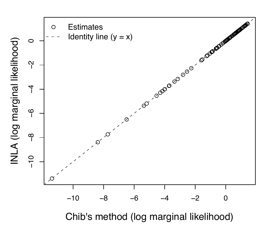
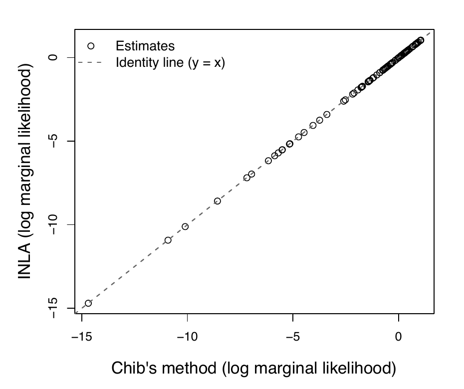
Table 2 reports numerical estimates across three standard prior standard deviations ( $\sigma_\beta \in \{1000, 10, 0.1\}$ ), including the exact benchmark, the INLA estimate, the mean and standard deviation across 5 Chib replications, and the INLA error against truth. INLA matches the analytical benchmark to within $0.0005$ – $0.0006$ log units in all settings, while the Monte Carlo standard error of Chib’s estimator is approximately $0.0002$ log units.

Table 2: Comparison of exact analytical marginal likelihood, INLA (integration-based), and Chib’s method ( $5$ replications with $100\,000$ iterations) for US crime data. The Monte Carlo standard error (MCSE) is $\text{SD}/\sqrt{5}$ .
$\mathcal{M}$	$\sigma_\beta$	Exact	INLA	Chib’s method ( $10^5$ iter)			Diff
5-7 (lr)8-8				Mean	SD	MCSE	( $\text{INLA} - \text{Exact}$ )
$\mathcal{M}_1$	1000	-73.2093	-73.2098	-73.2091	0.0006	0.0003	-0.0005
$\mathcal{M}_1$	10	-31.7733	-31.7739	-31.7735	0.0006	0.0003	-0.0005
$\mathcal{M}_1$	0.1	1.4380	1.4374	1.4379	0.0003	0.0001	-0.0006
$\mathcal{M}_2$	1000	-96.6376	-96.6381	-96.6375	0.0007	0.0003	-0.0005
$\mathcal{M}_2$	10	-41.3990	-41.3996	-41.3988	0.0003	0.0001	-0.0005
$\mathcal{M}_2$	0.1	1.0627	1.0621	1.0625	0.0003	0.0001	-0.0006

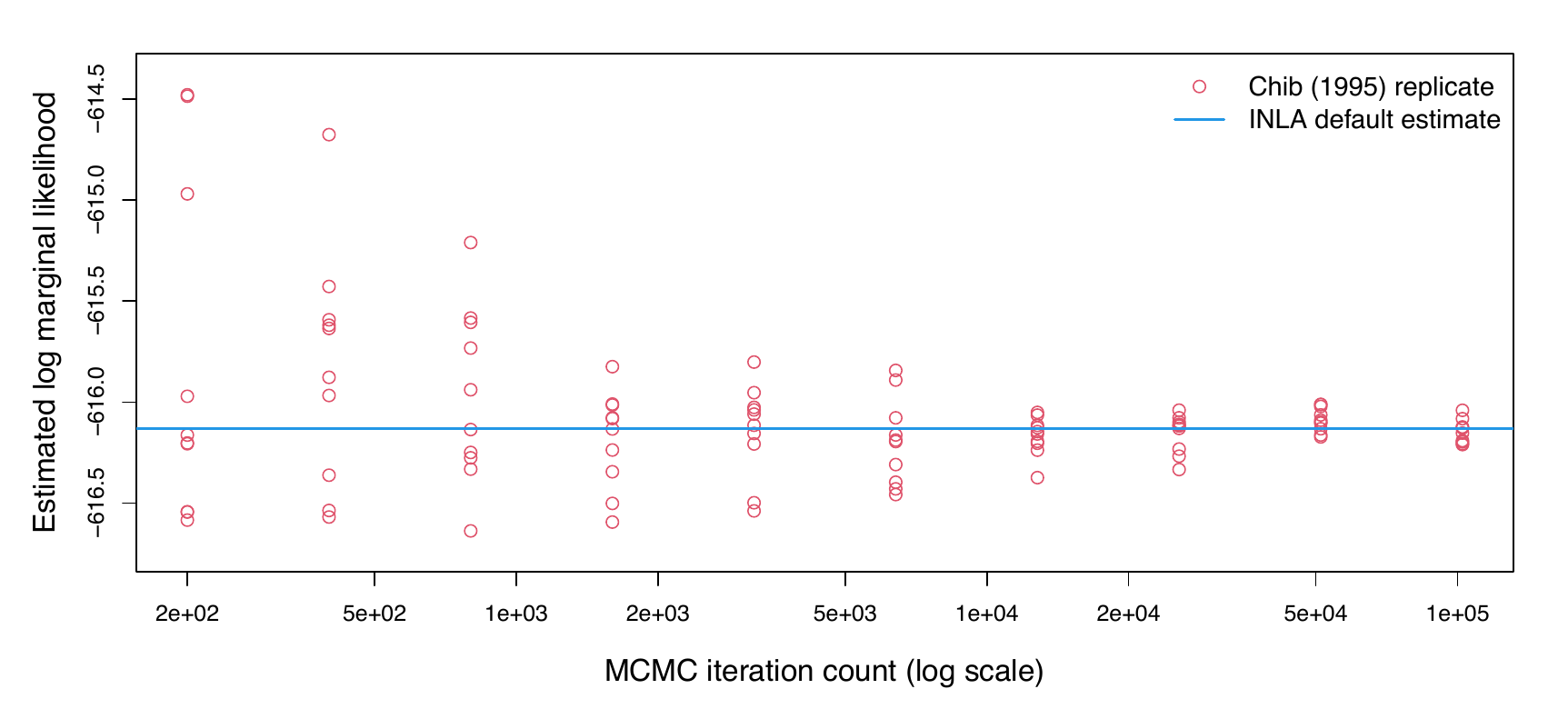
Going further into MCMC convergence, Figure 2 shows the performance of Chib’s method as a function of the number of iterations from $200$ to $102\,400$ ( $10$ independent replications per iteration level). The solid horizontal line indicates the INLA default estimate ( $-19.4768$ ) for model $\mathcal{M}_1$ under precision $\sigma_\beta^{-2} = 0.2$ . Crucially, the vertical axis in Figure 2 spans a very narrow interval of $[-19.494, -19.464]$ (a total span of only $0.030$ log units). Hence, the apparent scatter in the plot reflects microscopic Monte Carlo variation, which rapidly stabilizes around the deterministic INLA estimate as iterations increase. All 100 convergence runs use deterministic seeds $20000 + 100i + j$ ( $i, j \in \{1, \dots, 10\}$ ), recorded in results/seeds.csv.

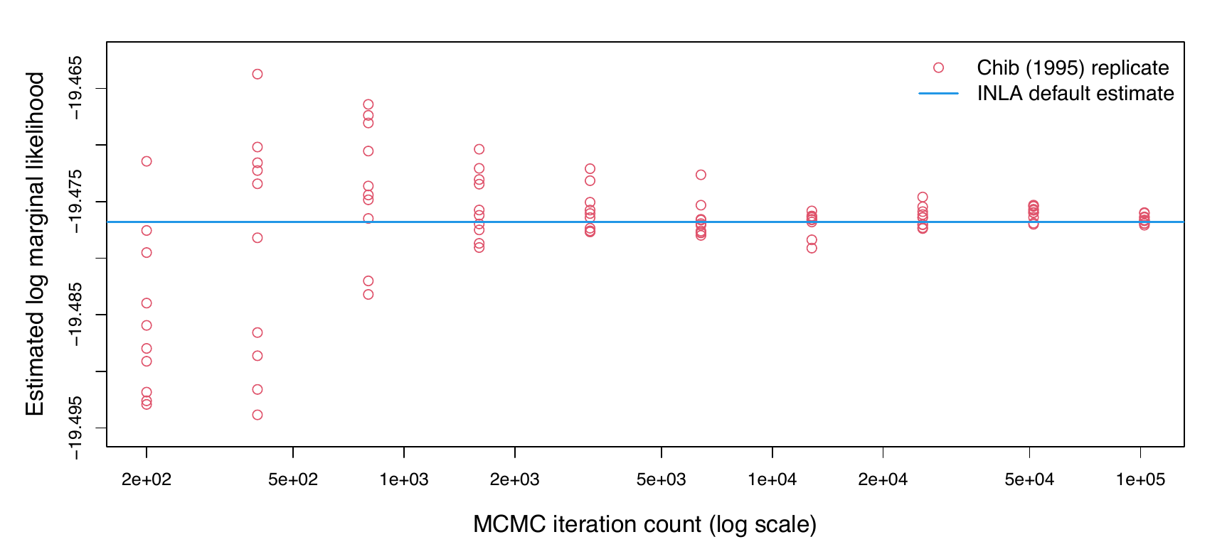
Fig 2: Convergence of Chib’s method across MCMC iteration counts ( $200$ to $102\,400$ , 10 runs per level) for the Gaussian regression model ( $\mu_\beta = 1, \sigma_\beta^{-2} = 0.2$ ). The horizontal line marks the default INLA estimate ( $-19.4768$ ). Note that the vertical axis spans only $0.030$ log units (from $-19.494$ to $-19.464$ ).

From Figure 2 one can see that Chib’s method requires substantial sampling effort to achieve high precision, whereas INLA returns a stable, near-exact value in a fraction of a second. The computational time for INLA is under 0.1 seconds for this model, while 100 000 iterations of Chib’s method require approximately 1.5 seconds per run on the same hardware.

INLA versus Chib’s method in probit regression

In the third example, we compare INLA with Chib’s method (Chib, 1995) for approximating the marginal likelihood in a Bayesian probit regression model $\mathcal{M}$ . The data set addressed is the simulated Bernoulli data introduced by Hubin & Storvik (2018). The model is given by $\begin{align} \begin{split} Y_t|\eta_t,\mathcal{M} \stackrel{iid}{\sim}& \text{Bernoulli}(\Phi(\eta_t));\\%\label{bernprobf}\\ \eta_t|\mathcal{M} =& \beta_0 + \sum_{i=1}^{p_{\mathcal{M} }} \beta_{i}x^{\mathcal{M}}_{ti};\\ \beta_i|\mathcal{M} \sim& N(\mu_\beta,\sigma_{\beta}^2),%\label{bernprobl}. \end{split} \end{align}$ where $t=1,...,2000$ and $i=0,...,p_{\mathcal{M}}$ . We addressed two different sets of explanatory variables with cardinalities 11 for model $\mathcal{M}_1$ and 13 for model $\mathcal{M}_2$ .

For Chib’s method, computations were performed using the MCMCprobit function in MCMCpack (Martin et al., 2011) with marginal.likelihood = "Chib95" and $100\,000$ iterations per replication across $5$ independent runs with fixed random seeds. For INLA, we used the binomial family with link = "probit", using strategy = "simplified.laplace" and int.strategy = "ccd". Since all prior precisions $\sigma_\beta^{-2}$ were fixed across evaluations, no further hyperparameter optimization over regression priors was required.

Table 3: Comparison of INLA and Chib’s method for Bayesian probit regression across 5 independent replications with $100\,000$ iterations. $\text{MCSE} = \text{SD}/\sqrt{5}$ .
$\mathcal{M}$	$\sigma_\beta$	INLA	Chib’s method ( $10^5$ iter, 5 reps)				Diff
4-7 (lr)8-8			Mean	SD	MCSE	Replicates	( $\text{INLA} - \text{Mean}$ )
$\mathcal{M}_1$	1000	-688.3190	-688.2854	0.0489	0.0219	-688.30, -688.29, -688.36, -688.23, -688.24	-0.0336
$\mathcal{M}_1$	10	-633.0900	-633.0655	0.0239	0.0107	-633.05, -633.03, -633.09, -633.09, -633.07	-0.0245
$\mathcal{M}_1$	0.1	-669.7585	-669.7517	0.0129	0.0058	-669.77, -669.75, -669.74, -669.75, -669.74	-0.0068
$\mathcal{M}_2$	1000	-704.2263	-704.1979	0.0466	0.0208	-704.27, -704.20, -704.14, -704.19, -704.18	-0.0285
$\mathcal{M}_2$	10	-639.8049	-639.7549	0.0522	0.0233	-639.68, -639.77, -639.78, -639.72, -639.82	-0.0500
$\mathcal{M}_2$	0.1	-649.7799	-649.7816	0.0310	0.0139	-649.81, -649.80, -649.78, -649.78, -649.73	$+0.0017$

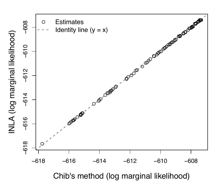
We used $\mu_\beta = 0$ , varying the prior precisions continuously between 0 and 10 in Figure 3, while Table 3 evaluates $\sigma_\beta \in \{1000, 10, 0.1\}$ (precisions $10^{-6}, 10^{-2}$ , and $10^2$ ), extending beyond the figure’s range to assess highly concentrated priors. In Figure 3, the identity reference line ( $y = x$ ) is included. Across the 100 evaluated precision values, the median absolute discrepancy between INLA and Chib’s method is $0.0193$ for $\mathcal{M}_1$ and $0.0321$ for $\mathcal{M}_2$ (95th percentiles $0.0692$ and $0.0818$ ), while the discrepancy in the log Bayes factor $\log \text{BF}_{12}$ has a median of $0.0350$ and a maximum of $0.1347$ log units.

Fig 3: Comparisons of marginal log-likelihood estimates obtained by Chib’s method ( $x$ -axis) and INLA ( $y$ -axis) for 100 different values of the precision parameter $\sigma_{\beta}^{-2} \in [0, 10]$ under 2 models with different numbers of covariates, with the identity reference line ( $y = x$ ).

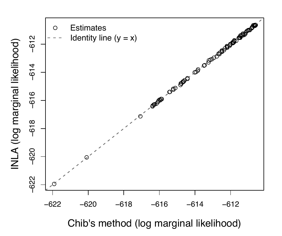
The computational time for INLA within these examples is under 0.2 seconds per model, whereas 100 000 iterations of Chib’s method required approximately 12.5 seconds per replication on the same hardware. Figure 4 displays the convergence of Chib’s estimator across MCMC iterations ( $200$ to $102\,400$ , with 10 independent replications per iteration level using deterministic seeds $40000 + 100i + j$ , $i, j \in \{1, \dots, 10\}$ , recorded in results/seeds.csv).

Fig 4: Convergence of Chib’s method across MCMC iteration counts ( $200$ to $102\,400$ , 10 runs per level) for probit regression ( $\mu_\beta = 1, \sigma_\beta^{-2} = 0.2$ ). The horizontal line marks the default INLA estimate ( $-616.1301$ ). Note that the vertical axis spans $2.16$ log units (from $-616.64$ to $-614.48$ ).

INLA versus other methods in logistic regression

In the fourth example we compare marginal likelihoods obtained by INLA with seven alternative evidence estimators benchmarked by Friel & Wyse (2012): standard Laplace approximation, Chib and Jeliazkov’s method, Laplace approximation at the MAP, harmonic mean estimator, power posteriors, annealed importance sampling (AIS), and nested sampling. The model $\mathcal{M}$ is the Bayesian logistic regression model with logit link addressed by Friel & Wyse (2012): $\begin{align} \begin{split} Y_t|\eta_t,\mathcal{M} \stackrel{iid}{\sim}& \text{Bernoulli}(\text{logit}^{-1}(\eta_t));\\%\label{bernprobf}\\ \eta_t|\mathcal{M} =&\beta_0 + \sum_{i=1}^{p_{\mathcal{M} }} \beta_{i}x^{\mathcal{M}}_{ti};\\ \beta_i|\mathcal{M} \sim& N(\mu_\beta,\sigma_{\beta}^2),%\label{bernprobl}. \end{split} \end{align}$ where $t=1,...,532$ and $i=0,...,p_{\mathcal{M}}$ . The data set addressed is the Pima Indians diabetes data ( $532$ complete records). For $\mathcal{M}_1$ , predictors comprise the number of pregnancies, plasma glucose concentration, body mass index, and diabetes pedigree function ( $p_{\mathcal{M}_1} = 4$ ); $\mathcal{M}_2$ additionally includes age ( $p_{\mathcal{M}_2} = 5$ ). All covariates were standardized to zero mean and unit variance. The models were evaluated under two prior variances: $\sigma_\beta^2 = 100$ and $\sigma_\beta^2 = 1$ with $\mu_\beta = 0$ .

Table 4 presents the results. Estimates for methods 3–9 are reproduced from the published benchmark of Friel & Wyse (2012) on the identical standardized dataset, where each Monte Carlo method used the equivalent of $200\,000$ samples. For INLA, we used strategy = "simplified.laplace" and int.strategy = "ccd" with fixed prior variances $\sigma_\beta^2 \in \{100, 1\}$ . To establish an independent ground truth, we also computed an importance sampling (IS) benchmark based on $200\,000$ draws from an inflated multivariate Student- $t_6$ proposal distribution centred at the posterior mode with scale matrix matching the inverse Hessian, achieving a Monte Carlo standard error of $\text{MCSE} = 0.003$ .

Table 4: Comparison of INLA, independent importance sampling reference, and seven baseline methods for logistic regression on Pima Indians data. Methods 3–9 are cited directly from the benchmark study of Friel & Wyse (2012). $\log \text{BF}_{12} = \log m(\mathbf{y}|\mathcal{M}_1) - \log m(\mathbf{y}|\mathcal{M}_2)$ .
	$\sigma_{\beta}^2 = 100$			$\sigma_{\beta}^2 = 1$
2-4 (lr)5-7 Method	$\mathcal{M}_1$	$\mathcal{M}_2$	$\log \text{BF}_{12}$	$\mathcal{M}_1$	$\mathcal{M}_2$	$\log \text{BF}_{12}$
INLA (classic mode)	-257.25	-259.89	2.64	-247.32	-247.59	0.27
Importance sampling (reference)	-257.23	-259.86	2.63	-247.30	-247.56	0.26
Laplace approximation	-257.26	-259.89	2.63	-247.33	-247.59	0.26
Chib and Jeliazkov	-257.23	-259.84	2.61	-247.31	-247.58	0.27
Laplace approximation MAP	-257.28	-259.90	2.62	-247.33	-247.62	0.29
Harmonic mean estimator	-284.78	-279.47	-5.31	-259.84	-260.55	0.71
Power posteriors	-257.98	-260.59	2.61	-247.57	-247.84	0.27
Annealed importance sampling	-257.87	-260.43	2.56	-247.30	-247.59	0.29
Nested sampling	-258.82	-261.38	2.56	-246.82	-246.97	0.15

A noticeable spread appears among the competing methods in Table 4: nested sampling sits $1.57$ log units below INLA for $\mathcal{M}_1$ under $\sigma_\beta^2 = 100$ and $0.50$ log units above INLA under $\sigma_\beta^2 = 1$ , while power posteriors and AIS differ by $0.6$ to $0.7$ log units. It is essential to address what this spread implies for applied inference. First, our independent importance sampling reference matches INLA within $0.02$ log units under both prior settings ( $-257.23$ vs. $-257.25$ at $\sigma_\beta^2 = 100$ , and $-247.30$ vs. $-247.32$ at $\sigma_\beta^2 = 1$ ), confirming that INLA’s Laplace approximation is near-exact for this GLM, whereas nested sampling and AIS exhibit small Monte Carlo underestimation biases under diffuse priors.

Second, because stochastic errors in nested sampling, power posteriors, and AIS are strongly positively correlated across models $\mathcal{M}_1$ and $\mathcal{M}_2$ , the discrepancy largely cancels on the decision-relevant scale of log Bayes factors. For $\sigma_\beta^2 = 100$ , INLA yields $\log \text{BF}_{12} = 2.64$ , compared to $2.63$ for IS, $2.63$ for Laplace, $2.61$ for Chib–Jeliazkov, $2.61$ for power posteriors, and $2.56$ for nested sampling and AIS, with a maximum across-method difference of only $0.08$ log units. Under $\sigma_\beta^2 = 1$ , all methods except the harmonic mean yield $\log \text{BF}_{12} \in [0.15, 0.29]$ , uniformly indicating that the evidence in favor of $\mathcal{M}_1$ is negligible. Thus, model-selection and model-averaging decisions are entirely preserved across methods. In terms of computational cost, INLA required under $0.05$ seconds, compared to substantial sampling budgets (200 000 evaluations) for the competing stochastic estimators (Friel & Wyse, 2012).

INLA versus Chib and Jeliazkov’s method in a Poisson mixed model

As models become more sophisticated, fewer methodologies are available for approximating the marginal likelihood. In the context of generalized linear mixed models (GLMMs), we consider the INLA approach (Rue et al., 2009) alongside the Metropolis–Hastings marginal likelihood estimator of Chib & Jeliazkov (2001) and the kernel density estimator of Chib et al. (1998).

This model analyzes epileptic seizure counts $Y_{jt}$ for $59$ patients measured first over an 8-week baseline period ( $t=0$ ) and subsequently across four 2-week follow-up periods ( $t=1,\dots,4$ ). After baseline, patients were randomized to either active treatment or placebo. Following standard practice for these data (Chib et al., 1998; Chib & Jeliazkov, 2001; Diggle et al., 1994), patient 49 (with an extreme baseline count of 151) was omitted as an outlier, leaving $58$ patients and $290$ total observations. The model $\mathcal{M}$ is specified as: $\begin{align} \begin{split} Y_{jt}|\eta_{jt},\mathcal{M} \sim& \text{Poisson}(\exp(\eta_{jt}));\\ \eta_{jt}|\mathcal{M} =& \log(\tau_{jt})+\beta_0 + \beta_1 x_{jt1} + \beta_2 x_{jt2} + \beta_3 x_{jt1}x_{jt2} + b_{j0} + b_{j1}x_{jt1};\\ \beta_i|\mathcal{M} \sim& N(0,100),\quad\quad i=0,...,3;\\ \mathbf{b}_j|\mathbf{D},\mathcal{M} \sim& N_2(0,\mathbf{D});\\ \mathbf{D}^{-1}|\mathcal{M} \sim& \text{Wishart}_2(4,I_2), \end{split} \end{align}$ for $j=1,...,58$ and $t=0,...,4$ . Here $x_{jt1} \in \{0,1\}$ indicates the post-baseline period, $x_{jt2} \in \{0,1\}$ denotes treatment assignment, $\tau_{jt}$ is the exposure offset ( $8$ for baseline, $2$ for visits), and $\mathbf{b}_j = (b_{j0}, b_{j1})'$ are patient-specific bivariate random effects with covariance matrix $\mathbf{D}$ .

In this example, the hyperparameter vector $\theta$ comprises the three non-redundant parameters of the precision matrix $\mathbf{D}^{-1}$ , meaning that numerical integration over hyperparameters requires three-dimensional quadrature. INLA produces both an integration-based estimate $\tilde{p}(\mathbf{y}|\mathcal{M})$ and a Gaussian approximation $\tilde{p}_G(\mathbf{y}|\mathcal{M})$ evaluated at the hyperparameter mode. Table 5 summarizes the estimates across different INLA approximation strategies (Gaussian, simplified Laplace, full Laplace) and integration schemes (CCD, grid, empirical Bayes), alongside the published MCMC reference values.

Table 5: Comparison of INLA marginal log-likelihood estimates across approximation strategies and hyperparameter integration schemes against literature MCMC benchmarks for the longitudinal Poisson GLMM on epileptic seizure counts.
Method / Strategy	Hyperparameter Integration	$\tilde{p}(\mathbf{y}\|\mathcal{M})$ (Integration)	$\tilde{p}_G(\mathbf{y}\|\mathcal{M})$ (Gaussian)
INLA (Default: Simplified Laplace)	CCD	-914.67	-915.62
INLA (Gaussian approximation)	CCD	-914.67	-915.62
INLA (Full Laplace)	CCD	-914.67	-915.62
INLA (Simplified Laplace)	Grid	-915.26	-915.62
INLA (Full Laplace)	Grid	-915.26	-915.62
INLA (Full Laplace)	Fine Grid ( $dz = 1.0$ )	-915.83	-915.62
INLA (Empirical Bayes mode)	None (EB)	-918.67	-915.62
Chib & Jeliazkov (2001) [JASA]	MCMC ( $10$ runs, $\text{SE} = 0.12$ )	-915.49
Chib, Greenberg & Winkelmann (1998)	MCMC (Kernel density)	-915.23

As shown in Table 5, the Gaussian approximation row $\tilde{p}_G(\mathbf{y}|\mathcal{M}) = -915.62$ reproduces the value of $-915.61$ reported in the initial preprint and agrees closely with Chib’s Metropolis–Hastings benchmark of $-915.49 \pm 0.12$ (Chib & Jeliazkov, 2001) and the kernel density estimate of $-915.23$ (Chib et al., 1998). Under default CCD integration over the 3-dimensional hyperparameter space, the integration-based estimate yields $-914.67$ . When switching to grid integration over $\theta$ , the integration estimate moves to $-915.26$ , and with a refined grid step ( $dz = 1.0$ ) reaches $-915.83$ , closely bracketing the MCMC benchmarks. Empirical Bayes (which omits the hyperparameter volume integration) underestimates the evidence at $-918.67$ . Note that in R-INLA, the strategy argument ("gaussian", "simplified.laplace", "laplace") governs the approximation of the univariate posterior marginals of the latent field, whereas the marginal likelihood in (6) always evaluates the Gaussian denominator $\tilde{\pi}_G(\boldsymbol{\eta}\vert{}\mathbf{y},\theta,\mathcal{M})$ at the mode $\boldsymbol{\eta}^*(\theta)$ ; consequently, $\tilde{p}(\mathbf{y}\vert{}\mathcal{M})$ in Tables 5 and 7 varies with the hyperparameter quadrature (int.strategy) rather than the latent marginal strategy.

This comparison offers a practical diagnostic rule for applied Bayesian practitioners: in mixed models with multiple hyperparameters, comparing the default CCD integration estimate against grid integration (or against the Gaussian approximation row) serves as an internal consistency check. A difference exceeding $0.5$ log units indicates that the hyperparameter posterior surface is moderately non-elliptical, and that grid integration or smaller step sizes should be selected. Across R-INLA releases, minor quadrature updates may slightly shift integration estimates (e.g., under R-INLA 25.06.07, the CCD estimate is $-914.77$ and grid is $-915.26$ , yielding a difference of $0.49$ log units). The $0.5$ log-unit threshold should therefore be understood as a practical rule-of-thumb rather than a sharp boundary. Importantly, this internal check specifically assesses the numerical stability and ellipticity of the hyperparameter integration over $\theta$ . It does not diagnose potential inaccuracies in the Laplace approximation of the latent field $\boldsymbol{\eta}$ itself, which must instead be evaluated by assessing the sample sizes and event counts per latent node. The computational time for INLA in this GLMM was approximately $1.8$ seconds for CCD integration and $12$ seconds for grid integration, compared to several minutes of MCMC sampling required for Chib’s estimator.

Decision-Scale Evaluation:
Bayes Factors and Model Probabilities

In applied model selection and Bayesian model averaging, what matters to the practitioner is not agreement to arbitrary decimal places, but whether approximation errors alter model selection decisions or distort posterior model probabilities $p(\mathcal{M}_k|\mathbf{y})$ in equations (3) and (4). In Table 6, we evaluate the discrepancy between INLA and reference estimators on the decision-relevant scale of log Bayes factors $\log \text{BF}_{12} = \log m(\mathbf{y}|\mathcal{M}_1) - \log m(\mathbf{y}|\mathcal{M}_2)$ and posterior model probabilities $P(\mathcal{M}_1|\mathbf{y})$ (assuming equal prior odds, $P(\mathcal{M}_1) = P(\mathcal{M}_2) = 0.5$ ). Evidence strength is categorized according to the standard interpretive scale of Kass & Raftery (1995): $|\log \text{BF}| < 1$ (barely worth mentioning), $1$ – $3$ (positive evidence), $3$ – $5$ (strong evidence), and $> 5$ (very strong evidence).

Table 6: Decision-scale comparison between INLA and reference benchmarks (Exact for US Crime, Chib for Probit, Importance Sampling for Pima). Across all scenarios, the absolute error in log Bayes factor satisfies $|\Delta \log \text{BF}| \le 0.026$ (within the Monte Carlo standard error of the MCMC reference), shifts posterior model probabilities by at most $0.002$ , and preserves the Kass & Raftery (1995) evidence categorization identically.
Dataset	Prior	$\log \text{BF}_{\text{Ref}}$	$\log \text{BF}_{\text{INLA}}$	$\Delta \log \text{BF}$	$P(\mathcal{M}_1\|\mathbf{y})_{\text{Ref}}$	$P(\mathcal{M}_1\|\mathbf{y})_{\text{INLA}}$	Evidence Category
US Crime	$\sigma_\beta = 1000$	23.428	23.428	$\phantom{-}0.000$	1.0000	1.0000	Very strong
US Crime	$\sigma_\beta = 10$	9.626	9.626	$\phantom{-}0.000$	0.9999	0.9999	Very strong
US Crime	$\sigma_\beta = 0.1$	0.375	0.375	$\phantom{-}0.000$	0.5927	0.5927	Not worth mentioning
Sim Probit	$\sigma_\beta = 1000$	15.912	15.907	-0.005	1.0000	1.0000	Very strong
Sim Probit	$\sigma_\beta = 10$	6.689	6.715	$+0.026$	0.9987	0.9988	Very strong
Sim Probit	$\sigma_\beta = 0.1$	-19.970	-19.979	-0.009	0.0000	0.0000	Very strong (for $\mathcal{M}_2$ )
Pima Logit	$\sigma_\beta^2 = 100$	2.626	2.636	$+0.010$	0.9325	0.9332	Positive
Pima Logit	$\sigma_\beta^2 = 1$	0.260	0.268	$+0.008$	0.5646	0.5666	Not worth mentioning

Table 6 demonstrates that across all eight evaluated regression scenarios, INLA’s error on the log Bayes factor scale never exceeds $0.026$ log units ( $0.010$ against exact and importance sampling benchmarks), and shifts posterior model probabilities by at most $0.002$ (two-tenths of one percent). In every single case, the scientific conclusion and the qualitative strength of evidence are completely identical to those obtained from the reference methods.

Probing the Limits:
Non-Gaussian and Small-Cluster Regimes

To further probe the boundaries of INLA’s marginal likelihood reliability, we designed two stress scenarios featuring known challenges for Laplace approximations:

Scenario S1 (Overdispersed Poisson GLMM): $n = 50$ observations generated with a low baseline rate ( $\beta_0 = -1.5, \beta_1 = 0.8, x_i \in [-1, 1]$ ), resulting in $68\%$ zeros, with an observation-level random effect $u_i \stackrel{\text{iid}}{\sim} N(0, \sigma_u^2)$ ( $\sigma_u = 0.7$ ). With small discrete counts, the Poisson likelihood is highly skewed, challenging the latent Gaussian assumption.
Scenario S2 (Small-Cluster Binary Logistic GLMM): $J = 20$ clusters of a very small size of 3, with binary response $Y_{jk} \sim \text{Bernoulli}(\text{logit}^{-1}(\beta_0 + \beta_1 x_{jk} + u_j))$ and substantial random intercept variance ( $\sigma_u = 1.2$ ). With only three binary trials per cluster, each latent variable $u_j$ is weakly identified and non-Gaussian.

In both scenarios, conditional on the fixed effects and hyperparameter $\tau_u = \sigma_u^{-2}$ , the latent variables are conditionally independent across clusters or observations. Consequently, the inner integral factors into a product of one-dimensional integrals, which can be evaluated to machine precision via $50$ -point Gauss-Hermite quadrature. Integrating the resulting conditional likelihood over $(\beta_0, \beta_1, \log \tau_u)$ on a fine $35 \times 35 \times 35$ adaptive grid provides a ground truth (error bounded with $< 10^{-4}$ ). Table 7 reports the results.

Table 7: Stress tests probing INLA marginal likelihood accuracy against 50-point Gauss-Hermite quadrature benchmarks under sparse, non-Gaussian regimes.
Scenario	INLA Configuration	INLA $\log m(\mathbf{y})$	Exact Reference	Discrepancy ( $\Delta$ )
S1: Low-Count Poisson	Default (Simplified Laplace + CCD)	-47.5829	-47.4815	-0.1014
(50 obs, 68% zeros, iid RE)	Gaussian Approximation	-47.5829	-47.4815	-0.1014
	Full Laplace + CCD	-47.5829	-47.4815	-0.1014
	Full Laplace + Grid	-47.6319	-47.4815	-0.1504
S2: Small-Cluster Binary	Default (Simplified Laplace + CCD)	-42.9984	-42.2332	-0.7652
(20 clusters of size 3, $N=60$ )	Gaussian Approximation	-42.9984	-42.2332	-0.7652
	Full Laplace + CCD	-42.9984	-42.2332	-0.7652
	Full Laplace + Grid	-42.9602	-42.2332	-0.7269

In Scenario S1, despite $68\%$ zero counts, INLA’s marginal likelihood approximation remains reasonably robust, incurring an underestimation bias of only $0.10$ to $0.15$ log units. In Scenario S2, however, the combination of binary outcomes and tiny cluster sizes of 3 pushes the Laplace approximation to its limits, resulting in a persistent underestimation of approximately $0.73$ to $0.77$ log units across all INLA configurations. This demonstrates that when binary data provide sparse information per latent Gaussian node, the Laplace approximation incurs a noticeable error.

Conclusions

The marginal likelihood is a cornerstone of Bayesian model selection, hypothesis testing, and model averaging. In this study, we conducted a systematic empirical evaluation of INLA’s marginal likelihood approximations against exact analytical benchmarks, converged MCMC estimators (Chib 1995, Chib and Jeliazkov 2001), independent importance sampling references, and thermodynamic competitors (Friel & Wyse, 2012).

Our findings indicate that for linear Gaussian models, probit and logit regressions, and GLMMs with moderate cluster sizes, INLA’s reported marginal likelihoods are remarkably accurate. On the decision-relevant scale of log Bayes factors, INLA’s discrepancies from reference benchmarks are negligible, which preserves scientific model-selection decisions without alteration. At the same time, INLA achieves speedups of two to three orders of magnitude over competing MCMC approaches.

However, our investigation also delineates the boundaries of this reliability. Under sparse latent structures, such as binary clustered data with very small cluster sizes, INLA’s Laplace approximation to the latent field can underestimate the marginal log-likelihood. Similarly, in mixed models featuring three or more hyperparameters, the default central composite design (CCD) integration can deviate from fine-grid or MCMC benchmarks. Consequently, modellers should routinely compare INLA’s default CCD integration estimate against grid integration or the Gaussian approximation row as an internal diagnostic check; a discrepancy exceeding $0.5$ log units indicates that the hyperparameter posterior surface is moderately non-elliptical and that grid integration or finer step sizes should be employed. Practitioners should recognize that this diagnostic isolates sensitivity to hyperparameter integration over $\theta$ ; it does not detect inaccuracies stemming from the Gaussian approximation $\tilde{\pi}_G(\boldsymbol{\eta} \mid \mathbf{y}, \theta, \mathcal{M})$ to the latent field in (6), which are governed by data discreteness and cluster sparsity.

When used with these diagnostics in mind, INLA provides a trustworthy, computationally formidable framework for Bayesian model selection and model averaging.

Data and Code Availability

Reproducibility Package: All code, datasets, and execution scripts are organized in a self-contained reproducibility package hosted at the canonical repository: https://github.com/aliaksah/INLA-marginal-likelihood. (The original exploratory scripts from 2016 remain archived at https://github.com/aliaksah/EMJMCMC2016). Across modern computational platforms (Apple Silicon ARM64 versus x86_64 Linux) and R-INLA releases, all stochastic estimators use fixed, logged random seeds (recorded in results/seeds.csv), and automated continuous integration workflows (.github/workflows/reproduce.yml) verify numerical reproducibility. A complete sessionInfo() environment log from R 4.4.1 and R-INLA 24.06.27 is archived in logs/. A comprehensive README.md and master driver script run_all.R are provided in the repository to map every script (00 through 05) directly to the generated tables, figures, and numerical logs.

Conflict of Interest Statement

The authors declare that they have no competing interests.

Acknowledgments

We would like to thank the CELS project at the University of Oslo and Integreat – Norwegian Centre for Knowledge-driven Machine Learning for giving us the opportunity, inspiration and motivation to write this article.

References

Berild, M. O., Martino, S., Gómez-Rubio, V., & Rue, H. (2022). Importance Sampling with the Integrated Nested Laplace Approximation. Journal of Computational and Graphical Statistics, 31(4), 1225–1237. https://doi.org/10.1080/10618600.2022.2067551 ↩
Chib, S. (1995). Marginal Likelihood from the Gibbs Output. Journal of the American Statistical Association, 90(432), 1313–1321. https://doi.org/10.1080/01621459.1995.10476635 ↩ 1 2 3
Chib, S., Greenberg, E., & Winkelmann, R. (1998). Posterior simulation and Bayes factors in panel count data models. Journal of Econometrics, 86(1), 33–54. https://doi.org/10.1016/s0304-4076(97)00108-5 ↩ 1 2 3
Chib, S., & Jeliazkov, I. (2001). Marginal Likelihood From the Metropolis–Hastings Output. Journal of the American Statistical Association, 96(453), 270–281. https://doi.org/10.1198/016214501750332848 ↩ 1 2 3 4 5 6
Diggle, P. J., Liang, K.-Y., & Zeger, S. L. (1994). Analysis of longitudinal data. Oxford University Press, Oxford. ↩
Friel, N., & Wyse, J. (2012). Estimating the evidence – a review. Statistica Neerlandica, 66(3), 288–308. https://doi.org/10.1111/j.1467-9574.2011.00515.x ↩ 1 2 3 4 5 6 7
Gómez-Rubio, V., Bivand, R. S., & Rue, H. (2020). Bayesian Model Averaging with the Integrated Nested Laplace Approximation. Econometrics, 8(2), 23. https://doi.org/10.3390/econometrics8020023 ↩
Hubin, A., & Storvik, G. (2018). Mode jumping MCMC for Bayesian variable selection in GLMM. Computational Statistics & Data Analysis, 127, 281–297. https://doi.org/10.1016/j.csda.2018.05.020 ↩ 1 2 3
Hubin, A., Storvik, G. O., Grini, P. E., & Butenko, M. A. (2020). A Bayesian Binomial Regression Model with Latent Gaussian Processes for Modelling DNA Methylation. Austrian Journal of Statistics, 49(4), 46–56. https://doi.org/10.17713/ajs.v49i4.1124 ↩
Jordan, M. I., Ghahramani, Z., Jaakkola, T. S., & Saul, L. K. (1999). An Introduction to Variational Methods for Graphical Models. Machine Learning, 37(2), 183–233. https://doi.org/10.1023/a:1007665907178 ↩
Kass, R. E., & Raftery, A. E. (1995). Bayes Factors. Journal of the American Statistical Association, 90(430), 773–795. https://doi.org/10.1080/01621459.1995.10476572 ↩ 1 2 3
López-Gómez, D., Gómez-Rubio, V., & García-Donato, G. (2026). Efficient model exploration with the integrated nested Laplace approximation. arXiv Preprint arXiv:2609.07283. ↩
Marin, J.-M., Pudlo, P., Robert, C. P., & Ryder, R. J. (2012). Approximate Bayesian computational methods. Statistics and Computing, 22(6), 1167–1180. https://doi.org/10.1007/s11222-011-9288-2 ↩
Martin, A. D., Quinn, K. M., & Park, J. H. (2011). MCMCpack : Markov Chain Monte Carlo in R. Journal of Statistical Software, 42(9). https://doi.org/10.18637/jss.v042.i09 ↩ 1 2
McGrory, C. A., & Titterington, D. M. (2007). Variational approximations in Bayesian model selection for finite mixture distributions. Computational Statistics & Data Analysis, 51(11), 5352–5367. https://doi.org/10.1016/j.csda.2006.07.020 ↩
Neal, R. M. (2008). The Harmonic Mean of the Likelihood: Worst Monte Carlo Method Ever. https://radfordneal.wordpress.com/2008/08/17/the-harmonic-mean-of-the-likelihood-worst-monte-carlo-method-ever/. ↩ 1 2 3 4
Newton, M. A., & Raftery, A. E. (1994). Approximate Bayesian Inference with the Weighted Likelihood Bootstrap. Journal of the Royal Statistical Society Series B: Statistical Methodology, 56(1), 3–26. https://doi.org/10.1111/j.2517-6161.1994.tb01956.x ↩
Raftery, A. E., Newton, M. A., Satagopan, J. M., & Krivitsky, P. N. (2007). Estimating the Integrated Likelihood via Posterior Simulation Using the Harmonic Mean Identity. In Bayesian Statistics 8 (pp. 371–416). Oxford University Press. https://doi.org/10.1093/oso/9780199214655.003.0015 ↩
Rue, H., Martino, S., & Chopin, N. (2009). Approximate Bayesian Inference for Latent Gaussian models by using Integrated Nested Laplace Approximations. Journal of the Royal Statistical Society Series B: Statistical Methodology, 71(2), 319–392. https://doi.org/10.1111/j.1467-9868.2008.00700.x ↩ 1 2
Tierney, L., & Kadane, J. B. (1986). Accurate Approximations for Posterior Moments and Marginal Densities. Journal of the American Statistical Association, 81(393), 82–86. https://doi.org/10.1080/01621459.1986.10478240 ↩
Vandaele, W. (1978). Participation in illegitimate activities: Ehrilich revisited. In Deterrence and Incapacitation: Estimating the Effects of Criminal Sanctions on Crime Rates (pp. 270–335). National Academy of Sciences, Washington, DC. ↩

Cite this article

Hubin, A., & Storvik, G. (2026). Estimating the marginal likelihood with Integrated nested Laplace approximation (INLA). Journal of Reproducible Statistics, 1, 9. https://doi.org/10.68365/jrepstat.2026.9

doi: https://doi.org/10.68365/jrepstat.2026.9

Downloads

PDF JATS XML .bib .ris .csl.json Reproducibility package (.zip) ef22672d80e9b4be6f5441a4e41e2d225203698324f3b1d0633fdca0bde02e2b

https://doi.org/10.68365/jrepstat.2026.9 also supports content negotiation, so reference managers can fetch the citation from the DOI directly. The exports above work without it.

Reproducibility record

Peer review record

Abstract

Introduction

INLA versus truth and the harmonic mean

INLA versus Chib’s method in Gaussian Bayesian regression

INLA versus Chib’s method in probit regression

INLA versus other methods in logistic regression

INLA versus Chib and Jeliazkov’s method in a Poisson mixed model

Decision-Scale Evaluation: Bayes Factors and Model Probabilities

Probing the Limits: Non-Gaussian and Small-Cluster Regimes

Conclusions

Data and Code Availability

Conflict of Interest Statement

Acknowledgments

References

Cite this article

Downloads

Decision-Scale Evaluation:
Bayes Factors and Model Probabilities

Probing the Limits:
Non-Gaussian and Small-Cluster Regimes